φ⁴ Theory and First Diagrams

The previous pages built the machinery: time ordering, Wick contractions, Gaussian generating functionals, functional derivatives, and Schwinger–Dyson identities. We now put those tools to work in the first genuinely interacting example: a real scalar field with a quartic self-interaction.

The interaction is simple enough to draw, but rich enough to teach nearly every organizational idea of perturbative QFT. A single vertex has four identical scalar legs. That one fact produces the first nontrivial combinatorics: vacuum bubbles, tadpoles, connected four-point functions, and symmetry factors. These diagrams are not decorative. They are a compact notation for terms in the Dyson expansion after Wick’s theorem has been applied.

The page keeps the external fields off shell and computes Green functions, not scattering amplitudes. This distinction matters: propagator corrections and connected four-point functions are the raw correlation functions from which physical amplitudes will later be extracted by amputation and on-shell limits.

The normalized interacting correlator

Non-normal-ordered phi-four interaction

We work in Lorentzian signature and define the interaction Hamiltonian density by

$$\mathcal H_I(x)=\frac{\lambda}{4!}\phi_I(x)^4,$$

so the Dyson factor is

$$\exp\left[-i\frac{\lambda}{4!}\int d^dy\,\phi_I(y)^4\right].$$

Equivalently, for a non-derivative interaction the Lagrangian interaction is $\mathcal L_I=-\lambda\phi^4/4!$. Throughout this page

$$G_0(x-y)=\langle 0|T\phi_I(x)\phi_I(y)|0\rangle, \qquad G_{ij}=G_0(x_i-x_j), \qquad G_{iy}=G_0(x_i-y).$$

The formulas below are for a non-normal-ordered $\phi^4$ interaction. If the interaction is replaced by $:\!\phi^4\!:$, the tadpole and one-vertex vacuum bubble terms discussed below are absent.

Let $|0\rangle$ be the free vacuum and $\phi_I$ the interaction-picture field. Under the vacuum-preparation assumptions stated below, the normalized interacting correlator is represented by

$$G_n(x_1,\ldots,x_n) = \frac{ \left\langle 0\left|T\phi_I(x_1)\cdots\phi_I(x_n) \exp\left[-i\frac{\lambda}{4!}\int d^dy\,\phi_I(y)^4\right]\right|0\right\rangle }{ \left\langle 0\left|T \exp\left[-i\frac{\lambda}{4!}\int d^dy\,\phi_I(y)^4\right]\right|0\right\rangle }.$$

This ratio uses the vacuum-preparation assumptions of the source-functional expansion: numerator and denominator share the switching, regulator and boundary prescription, and a literal ratio requires a nonzero denominator and a controlled interacting-vacuum switching limit. This is distinct from damping a fixed Hamiltonian. For a fixed self-adjoint Hamiltonian bounded below, shift the ground energy to zero and require nonzero projection of the boundary state onto a normalizable ground eigenspace; take long time at fixed damping before removing damping, specifying the selected ground-state components when that eigenspace is degenerate. The diagrams below are a formal expansion at a common regulator. Vacuum-bubble cancellation does not establish the switching limit or justify removal of the ultraviolet regulator.

The denominator is not a cosmetic normalization. It removes pieces in which part of the diagram is a vacuum bubble disconnected from the operator insertions. Without this division, an $n$-point function would contain extra factors describing vacuum fluctuations that occur independently of the fields being measured.

Expanding to first order gives

$$G_n(x_1,\ldots,x_n) =G_n^{(0)}(x_1,\ldots,x_n) -\frac{i\lambda}{4!}\int d^dy\, \Big[ \langle T\phi_1\cdots\phi_n\phi_y^4\rangle_0 - G_n^{(0)}\langle T\phi_y^4\rangle_0 \Big] +O(\lambda^2),$$

where $\phi_i=\phi_I(x_i)$, $\phi_y=\phi_I(y)$, and $\langle\cdots\rangle_0$ means a free-vacuum expectation value. The subtraction term is exactly the first-order effect of dividing by the denominator.

This formula is the first place where it becomes unavoidable to distinguish several ideas that are often compressed into the phrase “draw the diagram.” Wick’s theorem generates contractions. The Dyson expansion supplies powers of $-i\lambda$ and integrals over vertex positions. The normalization by $Z[0]$ cancels vacuum bubbles. What remains is organized by connectedness and by symmetry factors.

The φ⁴ vertex

The factor $1/4!$ in the interaction is chosen so that a vertex with four distinguishable external attachments carries the simple factor $-i\lambda$. In coordinate space the vertex position is integrated over; in momentum space the same integration will later become momentum conservation at the vertex.

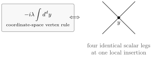
A $\phi^4$ insertion supplies four identical scalar fields at the same point $y$. The $4!$ possible attachments of four labeled external fields cancel the $1/4!$ in $\lambda\phi^4/4!$, leaving the coordinate-space vertex factor $-i\lambda\int d^dy$.

More explicitly, for four external fields there are $4!$ contractions connecting the four fields at $y$ to $\phi_1,\phi_2,\phi_3,\phi_4$. Therefore

$$-\frac{i\lambda}{4!}\int d^dy\, \langle T\phi_1\phi_2\phi_3\phi_4\phi_y^4\rangle_0 \supset -i\lambda\int d^dy\,G_{1y}G_{2y}G_{3y}G_{4y}.$$

This is the simplest connected interaction diagram in scalar field theory. It is also the cleanest example of why $\lambda\phi^4/4!$ is the natural normalization: the vertex factor is simple because the factorial has already paid for the permutations of identical fields at the vertex.

Vacuum bubbles and why they cancel

At first order, even the vacuum functional contains a nonzero term:

$$\langle T\phi_y^4\rangle_0=3G_0(0)^2.$$

Hence

$$Z[0]=1-\frac{i\lambda}{4!}\int d^dy\,3G_0(0)^2+O(\lambda^2) =1-\frac{i\lambda}{8}\int d^dy\,G_0(0)^2+O(\lambda^2).$$

Graphically this is a one-vertex vacuum bubble: the four fields at the vertex are paired into two loops. It is real QFT data about the vacuum energy, but it is irrelevant for normalized correlation functions of local operators. The division by $Z[0]$ removes all vacuum bubbles disconnected from the external insertions. This is why vacuum bubbles should not simply be erased from the theory; they are canceled in normalized correlators, while in contexts such as the cosmological constant or finite-temperature free energy they can become physically relevant.

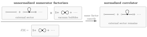
A vacuum bubble disconnected from the measured fields appears in the numerator, but the same factor appears in the denominator. Normalized Green functions keep diagrams connected to the operator insertions and discard purely vacuum factors.

The all-orders version is one of the most important bookkeeping facts in perturbation theory: disconnected vacuum bubbles exponentiate. Schematically,

$$Z[J]=e^{\text{vacuum bubbles}}\,Z_{\mathrm{with\ sources}}[J],$$

and the normalized functional $Z[J]/Z[0]$ cancels the vacuum-bubble exponential.

Two-point function: the tadpole

The first correction to the two-point function comes from

$$-\frac{i\lambda}{4!}\int d^dy\, \left[ \langle T\phi_1\phi_2\phi_y^4\rangle_0 -G_{12}\langle T\phi_y^4\rangle_0 \right].$$

Wick’s theorem gives two relevant classes of terms:

$$\langle T\phi_1\phi_2\phi_y^4\rangle_0 =3G_{12}G_0(0)^2+12G_{1y}G_{2y}G_0(0).$$

The first term is a free propagator times a vacuum bubble. It is canceled by the denominator. The second term is connected to the external fields. Its factor $12$ has a simple origin: choose one of the four fields at $y$ to contract with $\phi_1$, one of the remaining three to contract with $\phi_2$, and then contract the last two with each other.

Thus the first interacting correction is

$$\boxed{ G_2(x_1,x_2) =G_{12} -\frac{i\lambda}{2}\int d^dy\,G_{1y}G_{2y}G_0(0) +O(\lambda^2). }$$

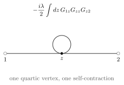
The tadpole correction to $G_2$ attaches two legs of the $\phi^4$ vertex to the external points and contracts the remaining two legs with each other. Its coefficient is $(-i\lambda/4!)\times 12=-i\lambda/2$.

The factor $G_0(0)$ is the propagator evaluated at coincident points. In continuum field theory it is typically ultraviolet divergent. This is the first warning that interacting fields need renormalization. At this stage, however, the important lesson is more elementary: interactions correct propagation because a field quantum can interact with vacuum fluctuations and then continue on its way.

In momentum space, the same diagram is independent of the external momentum at this order. It behaves like a correction to the mass term. Later, this contribution will be organized as part of the self-energy.

Four-point function: the first connected vertex

For a free Gaussian field, the four-point function is only a sum of pairings:

$$G_4^{(0)}(x_1,x_2,x_3,x_4) =G_{12}G_{34}+G_{13}G_{24}+G_{14}G_{23}.$$

The free connected four-point function is zero. This is precisely what it means for the free theory to be Gaussian: every higher correlation function is built from two-point functions.

The first connected four-point contribution appears at order $\lambda$:

$$\boxed{ G_{4,c}^{(1)}(x_1,x_2,x_3,x_4) =-i\lambda\int d^dy\, G_{1y}G_{2y}G_{3y}G_{4y}. }$$

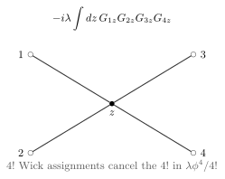
The first connected four-point function in $\phi^4$ theory has one integrated vertex. The $4!$ contractions of the four identical fields at the vertex cancel the $1/4!$ in the interaction.

The full normalized four-point function at order $\lambda$ also contains disconnected terms: a tadpole-corrected two-point function multiplied by a free two-point function. The connected part isolates the genuinely four-field correlation. Amputating the four tree-level external propagators leaves the vertex factor $-i\lambda$. When isolated stable one-particle poles with nonzero field overlap and the required asymptotic states exist, LSZ reduction supplies the on-shell scattering interpretation with the appropriate external-state normalization. In the convention $S=1+iT$, this tree contribution is $i\mathcal M=-i\lambda$, so the invariant amplitude is $\mathcal M=-\lambda$; see the scalar contact normalization check. Before reduction, the displayed expression remains an unamputated Green-function contribution.

Symmetry factors

The preceding examples suggest a compact rule. For a coordinate-space diagram in $\lambda\phi^4$ theory,

$$\text{contribution} = \frac{(-i\lambda)^V}{S_\Gamma} \int \prod_{a=1}^V d^dy_a\, \prod_{\text{lines }\ell}G_0(\ell),$$

where $V$ is the number of quartic vertices and $S_\Gamma$ is the symmetry factor of the diagram. Roughly speaking, $S_\Gamma$ counts permutations of identical internal lines and vertices that leave the diagram unchanged while the external labels are held fixed.

The examples above are:

$$S_{\text{four-point tree}}=1, \qquad S_{\text{tadpole}}=2, \qquad S_{\text{one-vertex vacuum bubble}}=8.$$

At second order in $\lambda$, the two-point function contains the first “sunset” topology:

$$\boxed{ G_{2,\mathrm{sunset}}^{(2)}(x_1,x_2) = \frac{(-i\lambda)^2}{6} \int d^dy\,d^dz\, G_{1y}G_0(y-z)^3G_{zx_2}. }$$

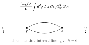
The sunset diagram has two quartic vertices and three identical internal propagators joining them. The final coefficient for the labeled two-point function is $(-i\lambda)^2/6$.

A quick way to see the factor is to count Wick contractions. Count labeled Wick contractions first; draw the unlabeled diagram only afterward. The Dyson expansion supplies $1/2!$ for the two vertices and $(1/4!)^2$ from the two interaction terms. The contractions give $2\cdot 4\cdot4\cdot3!$: either external point may attach to the first vertex, then one chooses a leg at each vertex for the two external fields, and then pairs the remaining three legs between the vertices. Therefore

$$\frac{1}{2!}\frac{1}{(4!)^2}\left(2\cdot4\cdot4\cdot3!\right)=\frac{1}{6}.$$

Symmetry factors are not mysterious constants attached to pictures by decree. They are the residue of Wick’s theorem after the obvious factorials in the exponential and in the interaction have canceled most, but not all, of the identical contractions.

Source-functional viewpoint

The same expansion can be generated without writing all Wick contractions by hand. Define the free source functional operationally by

$$Z_0[J]=\left\langle0\left|T\exp\left(i\int d^dx\,J(x)\phi_I(x)\right)\right|0\right\rangle,$$

so that field insertions are produced by $(1/i)\delta/\delta J(x)$. The interacting functional is

$$Z[J]=\exp\left[-i\frac{\lambda}{4!}\int d^dy\, \left(\frac{1}{i}\frac{\delta}{\delta J(y)}\right)^4\right]Z_0[J].$$

Normalized Green functions are obtained from

$$\mathcal Z[J]=\frac{Z[J]}{Z[0]}, \qquad G_n(x_1,\ldots,x_n) =\left. \frac{1}{i^n}\frac{\delta^n\mathcal Z[J]}{\delta J(x_1)\cdots\delta J(x_n)} \right|_{J=0}.$$

This formula is the algebraic engine behind the diagrams. Each functional derivative in the interaction vertex must land on a source from the Gaussian $Z_0[J]$. Lines are the free two-point functions produced by the Gaussian. Vertices are the interaction derivatives. Vacuum bubbles cancel because we use $\mathcal Z[J]$, not $Z[J]$. If a diagrammatic rule cannot be recovered from this labeled-source procedure, the rule has been remembered too vaguely.

Summary

The quartic scalar interaction is the first place where perturbation theory becomes visibly diagrammatic. The normalized interacting correlator is the Dyson expansion of the interaction-picture theory divided by the vacuum functional. Wick’s theorem turns each term into products of free propagators.

At first order, $\phi^4$ theory produces three basic lessons. A one-vertex vacuum bubble contributes to $Z[0]$ but cancels from normalized Green functions. A tadpole corrects the two-point function and already displays the ultraviolet sensitivity of coincident propagators. A one-vertex connected four-point function gives the first genuine interaction among four scalar insertions and becomes the tree-level $-i\lambda$ vertex after amputation.

The symmetry factor of a diagram is the leftover combinatorics after accounting for the factorials in the exponential and the interaction. Learning to compute these factors from Wick contractions is worth the effort: it prevents diagrams from becoming a mnemonic black box.

Common pitfalls

• The denominator in the normalized correlator is not optional. It cancels diagrams disconnected from the external insertions.
• A free four-point function is not connected. It is a sum of products of two-point functions.
• The $1/4!$ in $\lambda\phi^4/4!$ does not make the vertex small by a factor of $24$ in the four-point tree diagram; it cancels the $4!$ ways to attach the four legs.
• Tadpoles depend on whether the interaction is normal ordered. In $:\!\phi^4\!:$ perturbation theory, contractions among fields at the same vertex are removed.
• $G_0(0)$ is not an innocent finite number in continuum QFT. It is a regulated quantity whose divergence will later be absorbed into renormalized parameters.
• Symmetry factors depend on what is labeled. External points in a Green function are labeled; internal vertices are integrated and may be permuted.

Exercises

Exercise 1

Derive the first-order tadpole correction to the normalized two-point function in $\lambda\phi^4$ theory and show that its coefficient is $-i\lambda/2$.

Solution

Start from

$$G_2(x_1,x_2) =G_{12} -\frac{i\lambda}{4!}\int d^dy\, \left[ \langle T\phi_1\phi_2\phi_y^4\rangle_0 -G_{12}\langle T\phi_y^4\rangle_0 \right] +O(\lambda^2).$$

By Wick’s theorem,

$$\langle T\phi_y^4\rangle_0=3G_0(0)^2.$$

Also,

$$\langle T\phi_1\phi_2\phi_y^4\rangle_0 =3G_{12}G_0(0)^2+12G_{1y}G_{2y}G_0(0).$$

The first term cancels against the denominator subtraction. Therefore

$$G_2(x_1,x_2) =G_{12} -\frac{i\lambda}{4!}\int d^dy\,12G_{1y}G_{2y}G_0(0) +O(\lambda^2).$$

Since $12/4!=12/24=1/2$,

$$G_2(x_1,x_2) =G_{12} -\frac{i\lambda}{2}\int d^dy\,G_{1y}G_{2y}G_0(0) +O(\lambda^2).$$

Exercise 2

Show that the connected part of the first-order four-point function is

$$G_{4,c}^{(1)}(x_1,x_2,x_3,x_4) =-i\lambda\int d^dy\,G_{1y}G_{2y}G_{3y}G_{4y}.$$

Solution

The relevant first-order term is

$$-\frac{i\lambda}{4!}\int d^dy\, \langle T\phi_1\phi_2\phi_3\phi_4\phi_y^4\rangle_0.$$

The connected contribution is the class of contractions in which each external field is contracted with one field at the vertex $y$. There are $4!$ such contractions. Each produces

$$G_{1y}G_{2y}G_{3y}G_{4y}.$$

Thus

$$-\frac{i\lambda}{4!}\int d^dy\,4! G_{1y}G_{2y}G_{3y}G_{4y} =-i\lambda\int d^dy\,G_{1y}G_{2y}G_{3y}G_{4y}.$$

Other first-order terms either cancel as vacuum bubbles or factor into lower-point functions, so they do not contribute to the connected four-point function.

Exercise 3

Derive the symmetry factor $1/6$ of the sunset contribution to the labeled two-point function.

Solution

At order $\lambda^2$ the Dyson expansion gives

$$\frac{1}{2!}\left(-\frac{i\lambda}{4!}\right)^2 \int d^dy\,d^dz\, \langle T\phi_1\phi_2\phi_y^4\phi_z^4\rangle_0.$$

For the sunset topology, the two external fields attach to different vertices and the remaining three legs at $y$ are paired with the remaining three legs at $z$.

There are two choices for which external field attaches to $y$. Then there are $4$ choices for the leg at $y$ and $4$ choices for the leg at $z$. The remaining three legs can be paired in $3!$ ways. Hence the number of contractions is

$$2\cdot4\cdot4\cdot3!.$$

Multiplying by the expansion factors gives

$$\frac{1}{2!}\frac{1}{(4!)^2}\left(2\cdot4\cdot4\cdot3!\right) =\frac{1}{6}.$$

Therefore

$$G_{2,\mathrm{sunset}}^{(2)}(x_1,x_2) =\frac{(-i\lambda)^2}{6} \int d^dy\,d^dz\, G_{1y}G_0(y-z)^3G_{zx_2}.$$

Exercise 4

Suppose the interaction Hamiltonian density is $\mathcal H_I=\lambda:\!\phi^4\!:/4!$ instead of $\lambda\phi^4/4!$. Which of the first-order diagrams on this page survive?

Solution

Normal ordering removes contractions among fields inside the same interaction vertex. Therefore contractions of two fields at the same point $y$ inside $:\!\phi_y^4\!:$ are not allowed.

The one-vertex vacuum bubble requires pairing the four fields at $y$ among themselves, so it vanishes. The tadpole correction to the two-point function requires contracting two fields at $y$ with each other, so it also vanishes.

The connected four-point diagram survives. In that diagram, each of the four fields at $y$ contracts with one external field; there is no internal contraction within the same normal-ordered vertex. Thus

$$G_{4,c}^{(1)}(x_1,x_2,x_3,x_4) =-i\lambda\int d^dy\,G_{1y}G_{2y}G_{3y}G_{4y}$$

is unchanged.

References and further reading

• Sidney Coleman, Lectures of Sidney Coleman on Quantum Field Theory, Chapters 7–8, for the interaction picture, Dyson formula, Wick diagrams, and connected/disconnected diagrammatics.
• Mark Srednicki, Quantum Field Theory, Sections 8–10, for path-integral generating functionals and Feynman rules in interacting scalar field theory.
• A. Zee, Quantum Field Theory in a Nutshell, Chapter I.7, for a conceptual introduction to Feynman diagrams from source functionals.
• Michael E. Peskin and Daniel V. Schroeder, An Introduction to Quantum Field Theory, Sections 4.1–4.2, for perturbative Green functions and symmetry factors in $\phi^4$ theory.