Critical Behavior and Thermal Mass

The previous page explained why an Ising-like system near a continuous phase transition is naturally described by a Euclidean scalar field. The key parameter was the coefficient of $\phi^2$ : in the Gaussian approximation it is the square of the inverse correlation length, so a critical point is a massless limit.

This page asks what happens to that mass scale once the order-parameter field interacts with itself. The answer is the first field-theoretic lesson of critical phenomena: the coefficient of $\phi^2$ is not directly a physical inverse correlation length. It is shifted by fluctuations. The full zero-momentum inverse propagator is the inverse susceptibility, while the correlation length is defined by spatial decay. These quantities have the same zero at a continuous transition, but beyond the Gaussian approximation they need not be numerically equal.

The calculation is deliberately elementary. We study the one-loop tadpole correction in Euclidean $\phi^4$ theory and track how it depends on the ultraviolet cutoff $\Lambda$ , the infrared mass $m$ , and the spatial dimension $d$ . The result explains why mean-field theory works above four dimensions, why four dimensions is marginal, and why critical behavior in three dimensions requires renormalization-group ideas rather than ordinary perturbation theory.

A useful warning: this page is not trying to compute accurate critical exponents. It is teaching the diagnostic. When the loop correction becomes as sensitive to the long-distance scale as the tree-level term, ordinary perturbation theory has started to fail and the renormalization group must take over.

Correlation length, susceptibility, and the critical point

The Landau–Ginzburg functional for an Ising-like order parameter is

\mathcal F[\phi] =\int d^dx\left[ {1\over2}(\nabla\phi)^2 +{1\over2}r_0(T)\phi^2 +{\lambda\over4!}\phi^4 +\cdots \right].

The parameter $r_0(T)$ is often called a bare mass squared. In mean-field theory one writes

r_0(T)=a_0(T-T_0), \qquad a_0>0,

so the Gaussian propagator is

G_0(k)={1\over k^2+r_0(T)}.

If the theory were exactly Gaussian, the correlation length would be

\xi_0={1\over \sqrt{r_0(T)}}.

The transition would occur at $T=T_0$ , where $r_0(T_0)=0$ . But in an interacting theory this is too naive. First separate quantities that coincide only in the simplest approximation. The exponential correlation length is defined by the leading large-distance decay of the connected correlator,

G_c(x;T)\sim e^{-|x|/\xi_{\mathrm{exp}}(T)} \qquad (|x|\to\infty),

or, more generally, by the nearest singularity after analytic continuation in spatial momentum. The zero-momentum inverse propagator is instead

\boxed{ r_R(T)\equiv G^{-1}(0;T)=\chi_J^{-1}(T), \qquad m_\xi(T)\equiv\xi_{\mathrm{exp}}^{-1}(T). }

The analytic small-momentum expansion defines a different, second-moment length:

\begin{aligned} \xi_{\mathrm{2nd}}^2 &={1\over 2d\,\chi_J} \int d^dx\,|x|^2G_c(x),\\[2mm] G^{-1}(k;T) &=r_R(T)\left[1+\xi_{\mathrm{2nd}}^2(T)k^2+O(k^4)\right]. \end{aligned}

Here $\chi_J\equiv\partial\langle\phi\rangle/\partial J=G(0)$ is the susceptibility with respect to the source $J$ coupled to the chosen normalization of the order parameter. A physical magnetic susceptibility can differ by factors of $\beta$ and by field-normalization factors, as explained on the previous page.

In an interacting theory, $\xi_{\mathrm{2nd}}$ and $\xi_{\mathrm{exp}}$ need not have the same amplitude, although they diverge with the same exponent $\nu$ at an ordinary continuous transition. At Gaussian level, and at one-loop tadpole order on this page, the propagator has the single-pole form $G(k)=1/(k^2+r_R)$ . Then $\xi_{\mathrm{2nd}}=\xi_{\mathrm{exp}}=r_R^{-1/2}$ . Only in that approximation may one identify $G^{-1}(0)$ directly with $\xi_{\mathrm{exp}}^{-2}$ . Near a non-Gaussian fixed point, $\chi_J\sim\xi_{\mathrm{exp}}^{\,2-\eta}$ instead. Below we write $\xi$ for $\xi_{\mathrm{exp}}$ when only critical scaling is at issue.

The critical temperature is not the point where the bare parameter vanishes. It is the point where the correlation length diverges and the inverse susceptibility vanishes:

\boxed{ \begin{gathered} m_\xi(T_c)=0, \qquad r_R(T_c)=G^{-1}(0;T_c)=0,\\ \xi_{\mathrm{2nd}}(T_c)=\infty. \end{gathered} }

This distinction is the statistical-mechanical version of mass renormalization. The bare parameter is a coordinate in the microscopic theory. The correlation length and thermodynamic susceptibility are the long-distance observables.

The related long-distance quantities in this discussion play different roles:

Quantity	Meaning	Directly observable from long-distance correlations?
$r_0(T)$	bare quadratic coefficient in the cutoff theory	No
$r_R(T)=G^{-1}(0;T)=\chi_J^{-1}$	inverse source-normalized susceptibility	As a response, once that normalization is fixed
$m_\xi=\xi_{\mathrm{exp}}^{-1}$	inverse exponential correlation length from spatial decay	Yes
$\xi_{\mathrm{2nd}}$	second-moment length from the curvature of $G(k)$ at $k=0$	Yes

Keeping this distinction visible prevents a common mistake: treating a cutoff-dependent bare parameter as if it were the measured critical mass.

The discussion in this section is the symmetric-phase description above the transition. Below the transition, for an Ising-like one-component order parameter, the useful expansion is around one of the two minima rather than around $\phi=0$ . There is no Goldstone mode for a broken discrete $\mathbb Z_2$ symmetry, but the curvature at the chosen minimum still determines a correlation length.

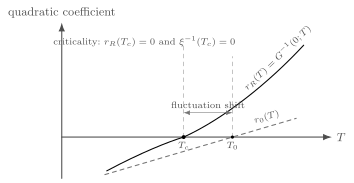
Bare quadratic coefficient and renormalized inverse susceptibility as functions of temperature — The transition occurs when the renormalized inverse susceptibility $r_R(T)=G^{-1}(0;T)$ vanishes. Interactions shift this zero from the naive Gaussian value $T_0$ to $T_c$ . The same point has $\xi_{\mathrm{exp}}^{-1}=0$ , although $G^{-1}(0)$ and $\xi_{\mathrm{exp}}^{-2}$ are not generally identical away from the Gaussian approximation.

Near the critical point it is conventional to define the reduced temperature

t={T-T_c\over T_c}.

Mean-field theory predicts

r_R\propto m_\xi^2\propto T-T_c, \qquad \xi\propto |T-T_c|^{-1/2}.

The exponent $1/2$ is the mean-field value of the correlation-length exponent $\nu$ . The rest of the page explains why this value is not generally reliable in dimensions below four.

Locality and the derivative expansion

The continuum functional is not just the few terms written above. Symmetry and locality allow an infinite series:

\mathcal F[\phi] =\int d^dx\left[ {1\over2}r_0\phi^2 +{1\over2}(\nabla\phi)^2 +{\lambda\over4!}\phi^4 +c_6\phi^6 +{c_{2,2}\over \Lambda^2}(\nabla^2\phi)^2 +{c_{4,2}\over \Lambda^2}\phi^2(\nabla\phi)^2 +\cdots \right].

The cutoff $\Lambda$ remembers the microscopic lattice spacing $a$ through $\Lambda\sim a^{-1}$ . Higher-derivative terms are suppressed at long wavelengths because every derivative brings a power of $k/\Lambda$ . For example,

{(\nabla^2\phi)^2/\Lambda^2\over (\nabla\phi)^2} \sim {k^2\over \Lambda^2}.

Thus, when $k\ll \Lambda$ , the leading long-distance physics is governed by the smallest number of derivatives and the most relevant powers of the field. This is why the same $\phi^4$ theory describes many different microscopic models in the Ising universality class.

The gradient term also explains how the lattice picture turns into a field theory. A nearest-neighbor cost such as

\sum_{x,\delta} (\phi_{x+\delta}-\phi_x)^2

becomes, after expanding at small lattice spacing,

\int d^dx\left[ C_1(\nabla\phi)^2 +{C_2\over \Lambda^2}(\nabla^2\phi)^2 +\cdots \right].

The first term is universal enough to survive in the minimal continuum model; the later terms are corrections to scaling.

The tadpole mass shift

Expand the interacting Euclidean functional around the symmetric phase. The tree-level propagator is

G_0(k)={1\over k^2+m^2},

where $m^2$ is the current infrared mass scale. At one loop, the quartic vertex can contract two of its four legs into a loop, leaving a correction to the two-point function. With the normalization $\lambda\phi^4/4!$ , the tadpole self-energy is

\boxed{ \Sigma_1(m) ={\lambda\over2} I_d(m;\Lambda), \qquad I_d(m;\Lambda) =\int_q^\Lambda {1\over q^2+m^2}. }

This term shifts the inverse propagator:

G^{-1}(k)=k^2+r_0(T)+\Sigma(k).

At one-loop tadpole order, $\Sigma(k)=\Sigma_1(m)$ is independent of $k$ . It therefore shifts the mass but not the coefficient of $k^2$ .

The symbol $m$ inside the loop should be read as the infrared mass used to regulate long-distance fluctuations. In strict perturbation theory it is the mass appearing in the propagator around which we expand. In a self-consistent or gap-equation treatment one sets it equal to the physical inverse correlation length. These are different approximations; the important lesson here is the scaling of the fluctuation correction near $m=0$ .

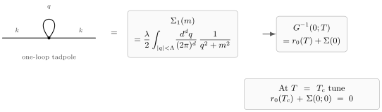
One-loop tadpole correction to the two-point function in Euclidean phi-four theory — The $\phi^4$ interaction gives a one-loop tadpole correction to the two-point function. In a statistical field theory this correction is a fluctuation-induced thermal mass shift, $\Sigma_1=(\lambda/2)\int_q^\Lambda 1/(q^2+m^2)$ .

The word “thermal” here should be read in the statistical-mechanical sense: the loop represents fluctuations of the order parameter in the Boltzmann ensemble. In finite-temperature quantum field theory, which appears on the next page, analogous loops are computed with Matsubara sums and give temperature-dependent masses. The logic is the same: fluctuations renormalize the quadratic term.

Evaluating the fluctuation integral

The integral

I_d(m;\Lambda) =\int_{|q|<\Lambda}{d^dq\over(2\pi)^d}{1\over q^2+m^2}

has both ultraviolet and infrared information. The ultraviolet part depends on the cutoff and shifts the microscopic relation between $r_0$ and $T$ . The infrared part depends on $m$ and controls the approach to criticality.

Using spherical coordinates in momentum space,

I_d(m;\Lambda) ={S_{d-1}\over(2\pi)^d} \int_0^\Lambda dq\,{q^{d-1}\over q^2+m^2},

where

S_{d-1}={2\pi^{d/2}\over \Gamma(d/2)}

is the area of the unit $(d-1)$ -sphere. For $2<d<4$ and $m\ll\Lambda$ , the cutoff term and the leading infrared nonanalytic term have the schematic form

I_d(m;\Lambda) =C_1\Lambda^{d-2}-A_dm^{d-2}+\cdots, \qquad 2<d<4,

with $A_d>0$ ; the sign is fixed because increasing $m^2$ decreases the integrand. For $d\le2$ , the integral at $m=0$ is already infrared singular in this Gaussian approximation, another sign that long-distance fluctuations cannot be treated casually near criticality.

For $d>4$ , the small- $m$ expansion begins instead with cutoff-dependent analytic terms,

I_d(m;\Lambda) =C_1\Lambda^{d-2}-D_dm^2\Lambda^{d-4}+\cdots,

with $D_d>0$ , before the infrared nonanalytic contribution proportional to $m^{d-2}$ (with logarithmic modifications at special even dimensions). The compact $m^{d-2}$ formula is therefore not the complete leading expansion above four dimensions.

In four dimensions, the expansion becomes

I_4(m;\Lambda) ={1\over16\pi^2}\left[ \Lambda^2 -m^2\log{ \Lambda^2+m^2\over m^2} \right],

so for $m\ll\Lambda$ ,

I_4(m;\Lambda) ={\Lambda^2\over16\pi^2} -{m^2\over16\pi^2}\log{\Lambda^2\over m^2} +\cdots.

The quadratic divergence is not itself the mystery. It is absorbed into the definition of the critical temperature. The logarithm is more interesting: it announces that $d=4$ is marginal for $\phi^4$ theory.

A useful way to see the special role of four dimensions is to differentiate the integral with respect to $m^2$ :

{\partial I_d\over \partial m^2} =-\int_q^\Lambda {1\over(q^2+m^2)^2}.

For momenta of order $q\sim m$ , dimensional analysis gives

\int {d^dq\over(q^2+m^2)^2} \sim m^{d-4}.

Thus the slope of the mass correction diverges as $m\to0$ for $d<4$ , has a logarithmic singularity at $d=4$ , and remains finite for $d>4$ .

This reproduces the route emphasized in the manuscript. In the Gaussian estimate $m_\xi^2\propto t$ , where $t=(T-T_c)/T_c$ , so the infrared part of the tadpole behaves for $2<d<4$ as

\left|\delta r_{\rm loop}^{\rm IR}\right| \sim \lambda m_\xi^{d-2} \sim \lambda t^{(d-2)/2}.

Compared with the tree term $r\sim t$ , its relative size is

{\left|\delta r_{\rm loop}^{\rm IR}\right|\over |r|} \sim \lambda t^{(d-4)/2}.

It grows on approaching criticality for $d<4$ , becomes logarithmic at $d=4$ , and shrinks for $d>4$ after local cutoff-dependent terms have been absorbed into the parameters. This is a diagnostic of the Gaussian fixed point, not an exact computation of the interacting critical exponents.

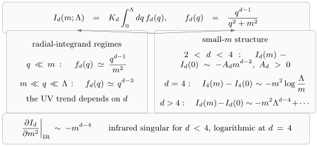
Scaling of the one-loop fluctuation integral with cutoff and infrared mass — The radial integrand crosses from $q^{d-1}/m^2$ in the deep infrared to $q^{d-3}$ for $m\ll q\ll\Lambda$ ; whether it rises or falls at large $q$ therefore depends on $d$ . The infrared part of its mass derivative scales as $m^{d-4}$ , so the critical point is perturbatively singular for $d\le4$ .

Critical temperature as a renormalization condition

At tadpole order, the renormalized inverse susceptibility is

r_R(T) =G^{-1}(0;T) =r_0(T)+\Sigma(0;m_\xi)+\cdots.

The critical point is defined by $r_R(T_c)=0$ and $m_\xi(T_c)=0$ , so

0=r_0(T_c)+\Sigma(0;0)+\cdots.

For $d>2$ , where $I_d(0;\Lambda)$ is infrared finite, the one-loop condition reads

0=r_0(T_c)+{\lambda\over2}I_d(0;\Lambda)+\cdots.

This equation determines the shift from the naive critical temperature $T_0$ to the true critical temperature $T_c$ . Since $I_d(0;\Lambda)$ is cutoff-dependent, the bare parameter $r_0(T)$ must also be cutoff-dependent if the physical critical temperature is to remain fixed.

It is often better to subtract the critical equation. Define a renormalized temperature variable $r(T)$ by

r(T)=r_0(T)-r_0(T_c).

Then the subtracted one-loop equation is

\boxed{ r_R(T) =r(T)+{\lambda\over2}\left[I_d(m_\xi;\Lambda)-I_d(0;\Lambda)\right]+\cdots. }

Because the one-loop tadpole is momentum independent, the propagator retains the single-pole form $G^{-1}(k)=k^2+r_R$ at this order. Thus $\xi_{\mathrm{2nd}}=\xi_{\mathrm{exp}}$ and one may set $r_R=m_\xi^2$ in this particular gap equation. That equality is an approximation, not the exact definition of either correlation length. For $d\le2$ , keep an infrared regulator rather than using $I_d(0)$ directly.

The subtraction removes the leading cutoff-dependent shift in the transition temperature. Equivalently,

I_d(m;\Lambda)-I_d(0;\Lambda) =-m^2\int_q^\Lambda {1\over q^2(q^2+m^2)}.

This difference is ultraviolet finite for $d<4$ , logarithmically divergent at $d=4$ , and power divergent for $d>4$ . The ultraviolet statement and the infrared statement are two sides of the same dimensional fact: $\lambda$ has engineering dimension

[\lambda]=4-d.

In four dimensions the coupling is dimensionless. Below four dimensions it becomes important at long distances. Above four dimensions it becomes less important at long distances.

The upper critical dimension

The previous paragraph can be turned into a simple scaling test about the Gaussian fixed point. At the scale of the correlation length, momenta are of order

k\sim \xi^{-1}=m_\xi.

The Gaussian estimate for the dimensionless strength of the quartic interaction at that scale is

g_\xi\sim \lambda \xi^{4-d} \sim \lambda m_\xi^{d-4}.

As $T\to T_c$ , the correlation length diverges. Therefore:

\begin{array}{ccl} d>4 &:& g_\xi\to0,\\ d=4 &:& g_\xi\text{ is marginal up to logarithms},\\ d<4 &:& g_\xi\to \infty. \end{array}

This is why $d_c=4$ is called the upper critical dimension of $\phi^4$ theory. Above four dimensions, mean-field theory becomes asymptotically correct at long distances. In four dimensions, logarithmic corrections appear. Below four dimensions, the fluctuations of the order parameter grow strong near the critical point and ordinary perturbation theory cannot be trusted.

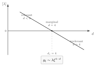
Dimensionless quartic coupling at the correlation-length scale — The Gaussian scaling estimate at the scale $\xi$ is $g_\xi\sim\lambda\xi^{4-d}$ . It decreases for $d>4$ , is marginal at $d=4$ , and grows away from the Gaussian fixed point for $d<4$ . This identifies $d_c=4$ as the upper critical dimension.

The manuscript gives a complementary four-point argument. Let

\mathcal B_d(k;\Lambda) =\int_{|q|<\Lambda}{d^dq\over q^2(q+k)^2}.

Its dimensional regimes are

\mathcal B_d(k;\Lambda)\sim \begin{cases} k^{d-4},&2<d<4,\\ \log(\Lambda/k),&d=4,\\ \Lambda^{d-4}+\text{local powers of }k +c_{\rm IR}k^{d-4}+\cdots,&d>4. \end{cases}

For $d\le2$ the massless bubble also needs an infrared regulator. Thus $k^{d-4}$ is the full leading scaling only in the infrared-finite range $2<d<4$ . At $d=4$ it is replaced by a logarithm, while above four dimensions the leading terms are local and cutoff dominated; the displayed nonlocal power has the usual logarithmic modifications at special even dimensions. After the local terms are absorbed into the renormalized coupling, the nonlocal infrared correction obeys

{\delta\lambda_{\rm IR}(k)\over\lambda} \sim \lambda k^{d-4},

which is the same dimensionless coupling obtained by setting $k\sim\xi^{-1}$ . For $d<4$ , the statement $g_\xi\to\infty$ describes the failure of perturbation theory about the Gaussian fixed point. The renormalization-group flow of the three-dimensional Ising universality class instead approaches a finite interacting Wilson–Fisher fixed point.

The same conclusion follows from the derivative of the tadpole integral. Near criticality,

{\partial \Sigma_1\over \partial m^2} =-{\lambda\over2}\int_q^\Lambda {1\over(q^2+m^2)^2} \sim -\lambda m^{d-4}.

For $d<4$ , this derivative becomes large as $m\to0$ . A small change in the mass produces a large fluctuation correction. That is the perturbative symptom of criticality.

What thermal mass means here

The term thermal mass can mean several related things, so it is worth being precise. The invariant long-distance scale on this page is the inverse correlation length

m_\xi(T)=\xi_{\mathrm{exp}}^{-1}(T),

while

r_R(T)=G^{-1}(0;T)=\chi_J^{-1}(T)

is the inverse susceptibility in the chosen order-parameter normalization. At Gaussian and one-loop tadpole level, the propagator is $G^{-1}(k)=k^2+r_R$ , so $\xi_{\mathrm{2nd}}=\xi_{\mathrm{exp}}$ and $r_R=m_\xi^2$ ; either quantity is therefore often called the thermal mass squared. Beyond that approximation the two correlation lengths can differ in amplitude, and $r_R$ scales differently from $m_\xi^2$ by the anomalous dimension.

Above the transition, $m_\xi>0$ and correlations decay exponentially:

G(x)\sim {e^{-|x|/\xi_{\mathrm{exp}}}\over |x|^{(d-1)/2}}, \qquad \xi_{\mathrm{exp}}={1\over m_\xi}.

At the transition, $m_\xi=0$ and the Gaussian theory gives a power law:

G(k)={1\over k^2}, \qquad G(x)\sim {1\over |x|^{d-2}}.

Interactions change the power law. At a nontrivial critical point, one writes

G(x)\sim {1\over |x|^{d-2+\eta}},

where $\eta$ is the anomalous-dimension exponent. Mean-field theory has $\eta=0$ and $\nu=1/2$ . In three-dimensional Ising-like systems these exponents are not equal to their mean-field values. The field theory still has the right variables, but the critical point is an interacting fixed point rather than a free Gaussian fixed point.

In finite-temperature relativistic QFT, “thermal mass” often refers to a mass shift induced by loops in a heat bath. The next page develops the imaginary-time formalism needed for such calculations. The present page is the static, long-distance prototype: an inverse correlation scale is renormalized by thermal fluctuations.

Summary

The coefficient of $\phi^2$ in a Landau–Ginzburg functional is a bare mass parameter. The inverse correlation length and inverse susceptibility are, respectively,

m_\xi=\xi_{\mathrm{exp}}^{-1}, \qquad r_R=G^{-1}(0)=\chi_J^{-1}.

At a continuous transition both vanish,

m_\xi(T_c)=0, \qquad r_R(T_c)=0,

but away from the Gaussian approximation one should not identify $r_R$ with $m_\xi^2$ . The transition is not determined by the vanishing of an arbitrary bare parameter.

The one-loop tadpole correction in Euclidean $\phi^4$ theory is

\Sigma_1(m)={\lambda\over2} \int^\Lambda {d^d q\over(2\pi)^d}\,{1\over q^2+m^2}.

It shifts the inverse susceptibility and hence shifts the critical temperature. At one-loop tadpole order, where the single-pole propagator gives $\xi_{\mathrm{2nd}}=\xi_{\mathrm{exp}}$ and $r_R=m_\xi^2$ , subtracting the critical value gives the schematic self-consistency condition

m_\xi^2(T) =r(T)+{\lambda\over2} \left[I_d(m_\xi)-I_d(0)\right]+\cdots.

The singular dependence of the loop integral on $m$ diagnoses the importance of fluctuations. Since

{\partial I_d\over\partial m^2}\sim -m^{d-4},

four dimensions is the upper critical dimension. Below four dimensions, critical fluctuations invalidate naive perturbation theory and force a renormalization-group treatment.

Common pitfalls

Identifying the bare zero with the critical point. The condition $r_0(T)=0$ is not generally the physical transition. Interactions shift the coefficient of $\phi^2$ , so the correct criterion is $G^{-1}(0;T_c)=0$ .
Treating a cutoff divergence as a universal prediction. The leading divergence in the tadpole integral renormalizes the location of $T_c$ . Universal information lives in the long-distance dependence on $m$ after the critical point has been fixed.
Extracting exact exponents from an unresummed one-loop gap equation. The tadpole computation is a diagnostic: it shows which fluctuations become large. In $d<4$ , reliable critical exponents require renormalization-group flow or another controlled nonperturbative method.
Mixing up dimensions. On this page $d$ is the dimension of the classical Euclidean statistical field theory. It is not the same symbol as the spacetime dimension of the Lorentzian QFT used earlier in the course.

Exercises

Exercise 1: the three-dimensional tadpole

Evaluate

I_3(m;\Lambda) =\int_{|q|<\Lambda}{d^3q\over(2\pi)^3}{1\over q^2+m^2}

and find its expansion for $m\ll\Lambda$ .

Solution

Use spherical coordinates:

I_3(m;\Lambda) ={4\pi\over(2\pi)^3} \int_0^\Lambda dq\,{q^2\over q^2+m^2} ={1\over2\pi^2} \int_0^\Lambda dq\,{q^2\over q^2+m^2}.

Rewrite

{q^2\over q^2+m^2}=1-{m^2\over q^2+m^2}.

Then

I_3(m;\Lambda) ={1\over2\pi^2}\left[ \Lambda-m\arctan{\Lambda\over m} \right].

For $m\ll\Lambda$ ,

\arctan{\Lambda\over m} ={\pi\over2}-{m\over\Lambda}+O\left({m^3\over\Lambda^3}\right),

I_3(m;\Lambda) ={\Lambda\over2\pi^2} -{m\over4\pi} +O\left({m^2\over\Lambda}\right).

The first term shifts the critical temperature. The second term is infrared-sensitive and nonanalytic in $m^2$ .

Exercise 2: subtracting the critical mass

In $d=3$ , use the result of Exercise 1 to show that

I_3(m;\Lambda)-I_3(0;\Lambda) =-{m\over4\pi}+O\left({m^2\over\Lambda}\right).

Then write the one-loop subtracted mass equation for $m=m_\xi$ .

Solution

From Exercise 1,

I_3(m;\Lambda) ={\Lambda\over2\pi^2} -{m\over4\pi} +O\left({m^2\over\Lambda}\right).

At $m=0$ ,

I_3(0;\Lambda)={\Lambda\over2\pi^2}.

Therefore

I_3(m;\Lambda)-I_3(0;\Lambda) =-{m\over4\pi}+O\left({m^2\over\Lambda}\right).

With interaction $\lambda\phi^4/4!$ , the subtracted one-loop equation is

m^2=r(T)+{\lambda\over2}\left[I_3(m)-I_3(0)\right]+\cdots.

Thus

m^2=r(T)-{\lambda\over8\pi}m+\cdots.

The term proportional to $m$ is more singular near $m=0$ than the Gaussian $m^2$ term. This does not give a trustworthy critical exponent by itself; it shows that naive perturbation theory breaks down near the three-dimensional critical point.

Exercise 3: identifying the upper critical dimension

Show by dimensional analysis that

\int {d^dq\over(q^2+m^2)^2} \propto m^{d-4}

for the infrared part of the integral. Use this to identify the upper critical dimension of $\phi^4$ theory.

Solution

Rescale the integration variable by $q=mp$ . Then

\int {d^dq\over(q^2+m^2)^2} =\int {m^d d^dp\over m^4(p^2+1)^2} =m^{d-4}\int {d^dp\over(p^2+1)^2}.

The remaining integral is dimensionless, up to ultraviolet issues. Therefore the infrared scaling is

\int {d^dq\over(q^2+m^2)^2} \sim m^{d-4}.

As $m\to0$ , this expression diverges for $d<4$ , becomes logarithmic for $d=4$ , and stays finite for $d>4$ . Thus $d_c=4$ is the upper critical dimension of $\phi^4$ theory.

Exercise 4: Ginzburg criterion from scaling

At the Gaussian fixed point in $d$ Euclidean dimensions, show that the engineering dimension of the scalar field is

[\phi]={d-2\over2},

and hence

[\lambda]=4-d.

Use this to argue that the dimensionless coupling at the scale $\xi$ is $g_\xi\sim \lambda\xi^{4-d}$ .

Solution

The kinetic term is

{1\over2}\int d^dx\,(\nabla\phi)^2.

The action or free-energy functional is dimensionless. Since $[d^dx]=-d$ and $[\nabla]=1$ , we need

-d+2+2[\phi]=0.

Therefore

[\phi]={d-2\over2}.

The interaction term is

\int d^dx\,{\lambda\over4!}\phi^4.

Its total dimension must vanish:

-d+[\lambda]+4[\phi]=0.

Substitute $[\phi]=(d-2)/2$ :

[\lambda]=d-4[\phi]=d-2(d-2)=4-d.

A coupling of mass dimension $4-d$ becomes dimensionless at the length scale $\xi$ after multiplication by $\xi^{4-d}$ :

g_\xi\sim \lambda\xi^{4-d}.

For $d<4$ , this grows as $\xi\to\infty$ , signaling strong critical fluctuations.

Exercise 5: mean-field correlation-length exponent

Assume fluctuations are negligible and

m_\xi^2(T)=A(T-T_c), \qquad A>0,

above the critical point. Find the correlation-length exponent $\nu$ defined by

\xi\sim (T-T_c)^{-\nu}.

Solution

By definition,

\xi={1\over m_\xi}.

m_\xi^2=A(T-T_c),

then

m_\xi=\sqrt{A}\,(T-T_c)^{1/2}.

Therefore

\xi={1\over\sqrt A}\,(T-T_c)^{-1/2}.

Thus the mean-field correlation-length exponent is

\nu={1\over2}.

Critical Behavior and Thermal Mass

Correlation length, susceptibility, and the critical point

Locality and the derivative expansion

The tadpole mass shift

Evaluating the fluctuation integral

Critical temperature as a renormalization condition

The upper critical dimension

What thermal mass means here

Summary

Common pitfalls

Exercises

Exercise 1: the three-dimensional tadpole

Exercise 2: subtracting the critical mass

Exercise 3: identifying the upper critical dimension

Exercise 4: Ginzburg criterion from scaling

Exercise 5: mean-field correlation-length exponent

Further reading