Operator Product Expansion in Perturbation Theory

The previous pages treated renormalization through vertices and masses. A hard loop was local when viewed from far away, so its effect could be absorbed into the coefficients of local operators. The operator product expansion is the local version of the same idea. Instead of asking how a loop corrects a vertex, we ask what happens when two local operators are brought close together.

The answer is not usually a single operator. It is an expansion:

$$\boxed{ \mathcal O_A(x)\mathcal O_B(0) \sim \sum_C C_{AB}^{\;C}(x)\mathcal O_C(0), \qquad x\to0. }$$

The coefficients $C_{AB}^{\;C}(x)$ are singular functions fixed by short-distance physics. The operators $\mathcal O_C$ carry the long-distance information. In a perturbative theory, Wick contractions let us calculate the coefficients explicitly. Once interactions are turned on, the same short-distance coefficients tell us which composite operators renormalize, which operators mix, and which logarithms appear in correlation functions.

This page develops the OPE in the simplest laboratory: the massless Euclidean scalar field in four dimensions, perturbed by $\lambda\phi^4/4!$. The goal is not merely to write formal expansions. The point is to see how the OPE reproduces two facts already encountered diagrammatically:

$${d\log Z_{\phi^2}\over dL}=-{\lambda\over16\pi^2}+O(\lambda^2), \qquad {d\lambda\over dL}=-{3\lambda^2\over16\pi^2}+O(\lambda^3),$$

where $L$ is an infrared coarse-graining time, $L=\log(\Lambda/k)$. Equivalently, with a renormalization scale $\mu$ increasing toward the ultraviolet,

$$\beta(\lambda)=\mu{d\lambda\over d\mu} ={3\lambda^2\over16\pi^2}+O(\lambda^3).$$

What the OPE means inside correlation functions

OPE normalization. The short-distance calculations below are Euclidean. We use the massless free propagator in four dimensions,

$$G(x)=\langle \phi(x)\phi(0)\rangle_0 =\int {d^4p\over(2\pi)^4}{e^{ip\cdot x}\over p^2} ={1\over4\pi^2x^2},$$

where $x^2=x_\mu x_\mu$. Composite operators are normal ordered with respect to this free propagator unless stated otherwise.

The two most important normalized operators on this page are

$$E(x)={1\over2}:\!\phi^2(x)\!:, \qquad U(x)={1\over4!}:\!\phi^4(x)\!:.$$

The interaction is

$$S_{\rm int}=\lambda\int d^4x\,U(x).$$

The factors $1/2$ and $1/4!$ are not cosmetic. They fix the numerical OPE coefficients that lead to the standard one-loop coefficient $3/(16\pi^2)$ for the $\phi^4$ beta function.

Local product versus integrated collision

The OPE itself is a statement about a local product at fixed separation $x$. Renormalization usually uses the integrated version. If two interaction insertions collide inside

$${\lambda^2\over2}\int d^4x\,d^4y\,U(x)U(y),$$

we change variables to a center coordinate $X$ and a relative coordinate $r=x-y$, then use the OPE only for the short-distance shell in $r$. The factor $1/2$ is the symmetry factor for the two identical interaction insertions; forgetting it doubles the beta function. The sign then comes from re-exponentiating the Euclidean weight $e^{-S}$: a positive local contribution to the expansion of $e^{-S}$ corresponds to a negative change in the coupling appearing in $S$.

The operator product expansion is an asymptotic statement inside correlation functions. Let

$$X=\mathcal O_1(y_1)\cdots\mathcal O_n(y_n)$$

be a collection of operators whose positions are far from the origin compared with $|x|$:

$$|x|\ll |y_i|.$$

Then the OPE means

$$\langle \mathcal O_A(x)\mathcal O_B(0)X\rangle \sim \sum_C C_{AB}^{\;C}(x) \langle \mathcal O_C(0)X\rangle.$$

The short-distance singularity in $x$ is universal for this local collision. The distant spectator operators only ask which local operator is produced at the origin.

At a scale-invariant fixed point, choose scalar scaling operators with dimensions $\Delta_A,\Delta_B,\Delta_C$. Dimensional analysis then fixes the leading scalar coefficient to have the form

$$\boxed{ C_{AB}^{\;C}(x) ={f_{AB}^{\;C}\over |x|^{\Delta_A+\Delta_B-\Delta_C}} }$$

up to tensor structures, descendant terms, and contact distributions. The constants $f_{AB}^{\;C}$ depend on operator normalization. Away from a fixed point the Wilson coefficients also depend on running couplings and can contain logarithms of the separation.

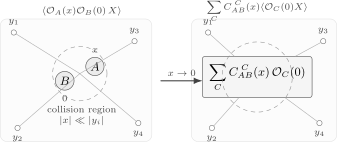
When two insertions are much closer to each other than to all other probes, their product can be replaced by a sum of local operators. The Wilson coefficients $C_{AB}^{\;C}(x)$ contain the short-distance singularity; the matrix elements of $\mathcal O_C$ contain the long-distance physics.

There are four important qualifications.

First, $\sim$ means an expansion as $x\to0$, not an ordinary Taylor series. In the generic perturbative setting used here it is interpreted asymptotically. In a Euclidean conformal field theory, radial quantization instead gives genuine OPE convergence whenever a sphere can separate the fused insertions from all spectator insertions.

Second, the OPE is local. It is not a statement about long-distance factorization. It is precisely the tool used when short distances become dangerous.

Third, the choice of operator basis matters. Multiplying an operator by a constant, adding total derivatives, or changing the subtraction scheme changes the numerical Wilson coefficients. Physical predictions are invariant only after coefficients and operator normalizations are used consistently.

Fourth, the OPE is a statement about distributions. Contact terms supported at coincident points can be invisible in separated-point correlators but essential in Ward identities, operator mixing, and renormalization of integrated insertions. When an operator is integrated over spacetime, these local contact terms cannot be omitted.

The free scalar OPE from Wick contractions

The simplest example is the free massless scalar field. Wick’s theorem gives

$$\phi(x)\phi(0)=G(x)\mathbf 1+:\!\phi(x)\phi(0)\!:.$$

The second term is nonsingular as $x\to0$, so we expand the remaining field around the origin:

$$\phi(x)=\phi(0)+x^\mu\partial_\mu\phi(0) +{1\over2}x^\mu x^\nu\partial_\mu\partial_\nu\phi(0)+\cdots.$$

Thus

$$\phi(x)\phi(0) \sim {1\over4\pi^2x^2}\mathbf 1 +:\!\phi^2(0)\!: +{x^\mu\over2}\partial_\mu:\!\phi^2(0)\!: +\cdots.$$

The identity operator is the most singular term. The next term is the local composite $:\!\phi^2\!:$, and then come derivative descendants and higher-dimension operators.

For normal-ordered monomials, the Wick combinatorics is especially transparent. At leading order in $x$, before writing derivative corrections,

$$\boxed{ :\!\phi^m(x)\!:\, :\!\phi^n(0)\!: \sim \sum_{r=0}^{\min(m,n)} {m\choose r}{n\choose r}r!\,G(x)^r :\!\phi^{m+n-2r}(0)\!: +\text{derivatives}. }$$

The integer $r$ counts the number of contractions connecting the two operators. Each cross-contraction contributes one factor of $G(x)$. Fields left uncontracted at $x$ are Taylor expanded to the origin.

A useful example is $E(x)E(0)$, where $E=:\!\phi^2\!:/2$. Wick contractions give

$$E(x)E(0) \sim {1\over2}G(x)^2\mathbf 1 +2G(x)E(0) +6U(0) +\text{derivatives and less singular terms}.$$

Substituting $G(x)=1/(4\pi^2x^2)$,

$$E(x)E(0) \sim {1\over32\pi^4x^4}\mathbf 1 +{1\over2\pi^2x^2}E(0) +6U(0)+\cdots.$$

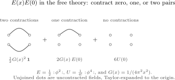
The free OPE of $E(x)E(0)$ is just Wick’s theorem organized by how many cross-contractions connect the two composite operators. Two contractions produce the identity coefficient, one contraction produces $E$, and zero contractions produce the local quartic operator $U$.

This calculation already shows the general logic. The most singular term is not always the term that matters for a given physical question. The identity coefficient controls disconnected short-distance singularities. The coefficient of $E$ controls how an $E$ insertion behaves under nearby fields. The coefficient of $U$ tells us that two thermal operators can produce the interaction operator.

For later comparison, here is the small amount of free-field algebra we will actually use:

Collision	Coefficient kept	Meaning
$E(x)E(0)$	${1\over2}G(x)^2\mathbf 1$	identity singularity in the two-point function
$E(x)E(0)$	$2G(x)E(0)$	thermal operator produced by a nearby thermal insertion
$E(x)E(0)$	$6U(0)$	two thermal insertions can make the quartic interaction
$U(x)E(0)$	${1\over2}G(x)^2E(0)$	one-loop renormalization of the thermal operator
$U(x)U(0)$	$3G(x)^2U(0)$	one-loop renormalization of the quartic coupling

The table is not a new principle; it is Wick’s theorem with the normalizations of $E$ and $U$ kept visible.

Composite operators and normal products

Products such as $\phi^2(x)$ and $\phi^4(x)$ are not automatically well-defined local quantum operators. Even in the free theory,

$$\langle \phi(x)^2\rangle_0=G(0)$$

is ultraviolet divergent. Normal ordering removes self-contractions at the same point:

$$:\!\phi^2(x)\!:=\phi^2(x)-G(0),$$

and similarly for higher powers. This is enough for free-field OPE calculations. It makes each operator finite before we collide it with another operator.

In an interacting theory, normal ordering is not the whole story. Interactions introduce new short-distance divergences when a composite insertion approaches an interaction vertex or another composite insertion. Those divergences are local, so they are removed by redefining composite operators as linear combinations of local operators with the same quantum numbers. Schematically,

$$\mathcal O_A^{\rm bare} =\sum_B Z_A^{\;B}\mathcal O_B^{\rm ren}.$$

This is operator renormalization. The OPE is the natural language for it because it tells us exactly which local operators can appear when short-distance points collapse.

For example, in the $\mathbb Z_2$-invariant scalar theory, even operators mix only with even operators. The operator $E\sim\phi^2$ can mix with the identity through additive vacuum terms and with total derivatives or equation-of-motion operators depending on the chosen basis. With a hard cutoff, $U\sim\phi^4$ can have power-sensitive mixing into lower-dimensional even operators such as $E$ and the identity. In a mass-independent scheme, logarithmic mixing is normally organized among operators of the same canonical dimension, together with total-derivative and equation-of-motion operators. Higher-dimensional operators are generated in the Wilsonian effective action, but that is distinct from logarithmic renormalization of a single $U$ insertion.

Endpoint logarithms in a composite two-point function

Consider the two-point function of the thermal operator $E=:\!\phi^2\!:/2$ at separation $R=|R|$ in the massless theory perturbed by

$$S_{\rm int}=\lambda\int d^4x\,U(x).$$

The free answer is

$$\langle E(0)E(R)\rangle_0 ={1\over2}G(R)^2 ={1\over32\pi^4R^4}.$$

At first order in $\lambda$,

$$\delta\langle E(0)E(R)\rangle =-\lambda\int d^4x\, \langle E(0)E(R)U(x)\rangle_0,$$

where the vacuum normalization gives no extra term because $U$ is normal ordered in the free theory.

The logarithmic divergence comes from two endpoint regions: $x$ close to $0$ and $x$ close to $R$. When $x$ is close to $0$, the relevant OPE is

$$U(x)E(0)\sim C_{UE}^{\;E}(x)E(0)+\cdots.$$

Using the Wick formula with $U=:\!\phi^4\!:/4!$ and $E=:\!\phi^2\!:/2$, the term that leaves an $E$ behind is obtained by contracting the two fields in $E$ with two of the four fields in $U$. There are

$${4\choose2}{2\choose2}2!=12$$

such contractions. Including the normalization factors gives

$$U(x)E(0) \sim {1\over2}G(x)^2E(0)+\cdots.$$

Therefore

$$C_{UE}^{\;E}(x)={1\over2}G(x)^2 ={1\over32\pi^4x^4}.$$

To keep the endpoint regions disjoint, choose a fixed $0<c<1/2$. Integrating near the origin over $\epsilon<|x|<cR$, where $\epsilon$ is a short-distance cutoff, gives

$$\int_{\epsilon<|x|<cR}d^4x\,C_{UE}^{\;E}(x) ={1\over32\pi^4}\,2\pi^2\int_\epsilon^{cR} {dr\over r} ={1\over16\pi^2}\log{R\over\epsilon} +\text{finite}.$$

The finite term is proportional to $\log c$ and does not affect the universal logarithmic coefficient.

The endpoint near $R$ gives the same contribution. Hence the logarithmic part of the first-order correction is

$$\boxed{ \delta\langle E(0)E(R)\rangle_{\log} =-{\lambda\over8\pi^2}\log{R\over\epsilon}\, \langle E(0)E(R)\rangle_0. }$$

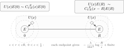
The first-order correction to $\langle E(0)E(R)\rangle$ has logarithmic endpoint regions. Near each endpoint, the OPE $U(x)E(0)\sim C_{UE}^{\;E}(x)E(0)$ turns the integration over the interaction vertex into a multiplicative renormalization of the local operator $E$.

This is exactly the OPE interpretation of the logarithmic factor used in the critical free-energy discussion. In the convention used here, define the multiplicative short-distance factor for each $E$ insertion by

$$Z_E(R,\epsilon)=1-{\lambda\over16\pi^2}\log{R\over\epsilon}+O(\lambda^2),$$

so two insertions produce twice the logarithm. If we write $L=\log(\Lambda/k)$, the infinitesimal form is

$${d\log Z_E\over dL}=-{\lambda\over16\pi^2}+O(\lambda^2).$$

Once the coupling itself runs, this differential equation is integrated with $\lambda=\lambda(L)$, producing the logarithmic powers discussed earlier.

Interaction fusion and the one-loop beta function

The same logic gives the one-loop beta function for the quartic interaction. We need the OPE of two interaction operators:

$$U(x)U(0), \qquad U={1\over4!}:\!\phi^4\!:.$$

From Wick contractions,

$$U(x)U(0) \sim {1\over24}G(x)^4\mathbf 1 +{1\over3}G(x)^3E(0) +3G(x)^2U(0) +\cdots.$$

The coefficient of $U(0)$ is the one that renormalizes the quartic coupling. Since

$$3G(x)^2={3\over16\pi^4x^4},$$

it is precisely logarithmic in four dimensions after integration over relative separation.

Now expand the interaction part of the Euclidean weight:

$$e^{-\lambda\int U} =1-\lambda\int d^4x\,U(x) +{\lambda^2\over2}\int d^4x\,d^4y\,U(x)U(y)+\cdots.$$

In the second-order term, focus on pairs with small separation

$$r=x-y, \qquad \epsilon<|r|<\epsilon e^{dL},$$

and center coordinate

$$X={x+y\over2}.$$

Using the OPE,

$${\lambda^2\over2} \int d^4X\int_{\epsilon<|r|<\epsilon e^{dL}}d^4r\,U\left(X+{r\over2}\right)U\left(X-{r\over2}\right)$$

contains

$${\lambda^2\over2} \int d^4X\,U(X) \int_{\epsilon<|r|<\epsilon e^{dL}}d^4r\,{3\over16\pi^4r^4}.$$

The shell integral is

$$\int_{\epsilon<|r|<\epsilon e^{dL}}d^4r\,{3\over16\pi^4r^4} ={3\over16\pi^4}2\pi^2dL ={3\over8\pi^2}dL.$$

Including the factor $1/2$ from the expansion gives

$${3\lambda^2\over16\pi^2}dL\int d^4X\,U(X).$$

This term appears with a plus sign in the expansion of $e^{-S}$. To rewrite the result as an effective action, compare

$$e^{-\lambda\int U} \left(1+{3\lambda^2\over16\pi^2}dL\int U\right) =\exp\left[-\left(\lambda-{3\lambda^2\over16\pi^2}dL\right)\int U+O(dL^2)\right].$$

Therefore the infrared Wilsonian flow is

$$\boxed{ {d\lambda\over dL}=-{3\lambda^2\over16\pi^2}+O(\lambda^3), \qquad L=\log{\Lambda\over k}. }$$

Equivalently, for a renormalized coupling defined at momentum scale $\mu$,

$$\boxed{ \beta(\lambda)=\mu{d\lambda\over d\mu} ={3\lambda^2\over16\pi^2}+O(\lambda^3). }$$

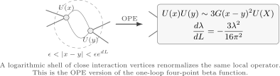
Two nearby interaction vertices fuse into a local interaction vertex. The coefficient of $U$ in the OPE $U(x)U(0)$ is logarithmic in four dimensions, and its shell integral gives the one-loop coefficient of the $\phi^4$ beta function.

This derivation is the same physics as the one-loop bubble calculation, reorganized locally. The bubble diagram says that hard internal momenta correct the local four-point vertex. The OPE says that two nearby interaction insertions produce the same local operator already present in the action. Same coefficient, different language.

Why logarithms are selected

The OPE makes the origin of logarithms almost too visible. In $d$ Euclidean dimensions, suppose

$$\mathcal O_A(x)\mathcal O_B(0) \supset {c\over |x|^d}\mathcal O_C(0).$$

Then integrating the relative separation over a short-distance shell gives

$$\int_{\epsilon}^{\epsilon e^{dL}} dr\,r^{d-1}{c\over r^d} =c\,dL$$

up to the angular volume of $S^{d-1}$. A coefficient with power $1/|x|^d$ is exactly marginal under the shell integration: it produces a logarithm.

More generally, if

$$\mathcal O_A(x)\mathcal O_B(0) \supset {c\over |x|^\alpha}\mathcal O_C(0),$$

then the shell integral behaves as

$$\int dr\,r^{d-1-\alpha}.$$

It is power divergent for $\alpha>d$, logarithmic for $\alpha=d$, and power suppressed for $\alpha<d$ as the shell shrinks. In the language of the RG, these are the local signals of relevant, marginal, and irrelevant short-distance fusion.

For $U=\phi^4/4!$ in $d=4$, the coefficient $U(x)U(0)\supset 3G(x)^2U(0)$ has precisely the form $1/x^4$. This is why the quartic coupling is marginal at tree level and runs logarithmically at one loop.

Summary

The operator product expansion is the statement that short-distance operator collisions can be replaced by a sum of local operators:

$$\mathcal O_A(x)\mathcal O_B(0) \sim \sum_C C_{AB}^{\;C}(x)\mathcal O_C(0).$$

In perturbation theory, the coefficients are computed by Wick contractions plus Taylor expansion. In the free scalar theory,

$$:\!\phi^m(x)\!:\, :\!\phi^n(0)\!: \sim \sum_r {m\choose r}{n\choose r}r!G(x)^r :\!\phi^{m+n-2r}(0)\!:+\cdots.$$

The coefficients of logarithmically singular terms are the local data that drive renormalization. For

$$E={1\over2}:\!\phi^2\!:, \qquad U={1\over4!}:\!\phi^4\!:,$$

we found

$$U(x)E(0)\sim {1\over2}G(x)^2E(0)+\cdots,$$

which gives

$${d\log Z_E\over dL}=-{\lambda\over16\pi^2}+O(\lambda^2),$$

and

$$U(x)U(0)\sim 3G(x)^2U(0)+\cdots,$$

which gives

$${d\lambda\over dL}=-{3\lambda^2\over16\pi^2}+O(\lambda^3).$$

Thus the OPE is not a separate topic from renormalization. It is the operator-level expression of locality in the ultraviolet.

Common pitfalls

Confusing normal ordering with the OPE. Normal ordering subtracts self-contractions inside one composite operator. The OPE studies singularities between two distinct insertions as their separation goes to zero.

Keeping only the most singular identity term. The identity term often controls disconnected divergences or vacuum-energy shifts. Coupling renormalization is controlled by the coefficient of the operator already present in the action.

Treating OPE coefficients as convention-free numbers. Rescaling $U$ or $E$ changes the coefficients. The physical statement is invariant only after the operator normalization and coupling normalization are fixed.

Reading the OPE as a large-distance expansion. It is a short-distance expansion used inside correlators whose other insertions remain far away.

Exercises

Exercise 1 — Wick-contraction combinatorics

Derive the free-theory Wick formula

$$:\!\phi^m(x)\!:\, :\!\phi^n(0)\!: \sim \sum_{r=0}^{\min(m,n)} {m\choose r}{n\choose r}r!\,G(x)^r :\!\phi^{m+n-2r}(0)\!: +\cdots.$$

Explain the combinatorial factor.

Solution

Because both monomials are normal ordered, contractions are only allowed between a field at $x$ and a field at $0$. Choose $r$ fields out of the $m$ fields in the first monomial and $r$ fields out of the $n$ fields in the second monomial. This gives

$${m\choose r}{n\choose r}$$

choices. Once the selected fields are chosen, pair them. There are $r!$ pairings. Each pairing contributes one free propagator $G(x)$, so $r$ pairings contribute $G(x)^r$.

After these contractions, there are $m-r$ uncontracted fields at $x$ and $n-r$ uncontracted fields at $0$. Taylor expanding the uncontracted fields at $x$ to the origin gives, at leading derivative order,

$$:\!\phi^{m+n-2r}(0)\!:.$$

Summing over $r$ gives the stated formula. The omitted terms are derivative descendants and less singular terms obtained from the Taylor expansion.

Exercise 2 — The free OPE of E with E

Using

$$E={1\over2}:\!\phi^2\!:, \qquad U={1\over4!}:\!\phi^4\!:,$$

show that

$$E(x)E(0) \sim {1\over2}G(x)^2\mathbf 1+2G(x)E(0)+6U(0)+\cdots.$$

Solution

Start with

$$:\!\phi^2(x)\!:\, :\!\phi^2(0)\!:.$$

The Wick formula has three terms.

For $r=2$, the coefficient is

$${2\choose2}{2\choose2}2!=2,$$

so the contribution is $2G(x)^2\mathbf 1$.

For $r=1$, the coefficient is

$${2\choose1}{2\choose1}1!=4,$$

so the contribution is

$$4G(x):\!\phi^2(0)\!:.$$

For $r=0$, the leading local term is

$$:\!\phi^4(0)\!:.$$

Now multiply by the normalization factor $1/2$ from each $E$, giving an overall factor $1/4$:

$$E(x)E(0) \sim {1\over4}\left[2G(x)^2\mathbf 1 +4G(x):\!\phi^2(0)\!: +:\!\phi^4(0)\!: \right]+\cdots.$$

Using $:\!\phi^2\!:=2E$ and $:\!\phi^4\!:=24U$, this becomes

$$E(x)E(0) \sim {1\over2}G(x)^2\mathbf 1 +2G(x)E(0) +6U(0)+\cdots.$$

Exercise 3 — Endpoint logarithms and thermal-operator renormalization

Compute the coefficient of $E(0)$ in the OPE $U(x)E(0)$ and use it to find the logarithmic endpoint correction to $\langle E(0)E(R)\rangle$ at first order in $\lambda$.

Solution

The term proportional to $E(0)$ comes from contracting both fields in $E(0)$ with two of the four fields in $U(x)$. The number of contractions is

$${4\choose2}{2\choose2}2!=12.$$

Thus

$$:\!\phi^4(x)\!:\, :\!\phi^2(0)\!: \supset 12G(x)^2:\!\phi^2(0)\!:.$$

Including the normalizations $U=:\!\phi^4\!:/4!$ and $E=:\!\phi^2\!:/2$, we get

$$U(x)E(0) \supset {12\over4!\,2}G(x)^2:\!\phi^2(0)\!: ={1\over4}G(x)^2:\!\phi^2(0)\!: ={1\over2}G(x)^2E(0).$$

Therefore

$$C_{UE}^{\;E}(x)={1\over2}G(x)^2={1\over32\pi^4x^4}.$$

The first-order correction is

$$-\lambda\int d^4x\,\langle E(0)E(R)U(x)\rangle_0.$$

The endpoint region near $0$ contributes

$$-\lambda\int_\epsilon^R d^4x\,C_{UE}^{\;E}(x) \langle E(0)E(R)\rangle_0 =-{\lambda\over16\pi^2}\log{R\over\epsilon}\, \langle E(0)E(R)\rangle_0.$$

The endpoint near $R$ gives the same contribution. Hence

$$\delta\langle E(0)E(R)\rangle_{\log} =-{\lambda\over8\pi^2}\log{R\over\epsilon}\, \langle E(0)E(R)\rangle_0.$$

Exercise 4 — Quartic fusion and the beta function

Show that the coefficient of $U(0)$ in $U(x)U(0)$ is $3G(x)^2$. Then derive

$${d\lambda\over dL}=-{3\lambda^2\over16\pi^2}$$

for $L=\log(\Lambda/k)$.

Solution

The term proportional to $:\!\phi^4\!:$ in

$$:\!\phi^4(x)\!:\, :\!\phi^4(0)\!:$$

comes from two cross-contractions. The number of such contractions is

$${4\choose2}{4\choose2}2!=6\cdot6\cdot2=72.$$

Therefore

$$:\!\phi^4(x)\!:\, :\!\phi^4(0)\!: \supset 72G(x)^2:\!\phi^4(0)\!:.$$

Including $U=:\!\phi^4\!:/4!$ on both sides,

$$U(x)U(0) \supset {72\over(4!)^2}G(x)^2:\!\phi^4(0)\!: ={72\over576}G(x)^2\,24U(0) =3G(x)^2U(0).$$

Since

$$G(x)^2={1\over16\pi^4x^4},$$

we have

$$3G(x)^2={3\over16\pi^4x^4}.$$

The second-order term in the expansion of the Euclidean weight is

$${\lambda^2\over2}\int d^4x\,d^4y\,U(x)U(y).$$

Using the OPE in a shell $\epsilon<|r|<\epsilon e^{dL}$ gives a contribution

$${\lambda^2\over2}\int d^4X\,U(X) \int_{\epsilon<|r|<\epsilon e^{dL}}d^4r\,{3\over16\pi^4r^4}.$$

The angular volume of $S^3$ is $2\pi^2$, so the shell integral is

$${3\over16\pi^4}2\pi^2dL={3\over8\pi^2}dL.$$

Thus the second-order term contributes

$${3\lambda^2\over16\pi^2}dL\int d^4X\,U(X)$$

to the expansion of $e^{-S}$. Re-exponentiating,

$$\lambda\mapsto \lambda-{3\lambda^2\over16\pi^2}dL,$$

so

$${d\lambda\over dL}=-{3\lambda^2\over16\pi^2}.$$

Exercise 5 — The dimensional criterion for a logarithm

In $d$ Euclidean dimensions, suppose an OPE contains

$$\mathcal O_A(x)\mathcal O_B(0) \supset {c\over |x|^\alpha}\mathcal O_C(0).$$

Classify the short-distance shell integral as power divergent, logarithmic, or power suppressed as the shell radius shrinks.

Solution

The shell integral over the relative coordinate has radial measure

$$d^dx=\Omega_{d-1}r^{d-1}dr,$$

so the relevant radial behavior is

$$\int dr\,r^{d-1-\alpha}.$$

If $\alpha>d$, then the exponent $d-1-\alpha<-1$, and the integral is power divergent as the lower cutoff goes to zero.

If $\alpha=d$, then

$$\int {dr\over r}$$

is logarithmic.

If $\alpha<d$, then the integral is finite as the lower cutoff goes to zero and the contribution from a shrinking shell is power suppressed.

Thus logarithms arise precisely when the OPE coefficient scales as $1/|x|^d$.

Further reading

• Polyakov, Alexander M. Gauge Fields and Strings. Chur: Harwood Academic Publishers, 1987.
• Srednicki, Mark. Quantum Field Theory. Cambridge: Cambridge University Press, 2007, Sections 26–29.
• Weinberg, Steven. The Quantum Theory of Fields. Volume II: Modern Applications. Cambridge: Cambridge University Press, 1996, Sections 18.1 and 18.8.
• Wilson, Kenneth G. “Non-Lagrangian Models of Current Algebra.” Physical Review 179, no. 5 (1969): 1499–1512.
• Wilson, Kenneth G., and John Kogut. “The Renormalization Group and the $\epsilon$ Expansion.” Physics Reports 12, no. 2 (1974): 75–199.
• Zimmermann, Wolfhart. “Normal Products and the Short Distance Expansion in the Perturbation Theory of Renormalizable Interactions.” Annals of Physics 77, no. 1–2 (1973): 570–601.
• Zinn-Justin, Jean. Quantum Field Theory and Critical Phenomena. 4th ed. Oxford: Clarendon Press, 2002, Chapters 8–13.

References

Section titled “References”- Schwartz, Matthew D. Quantum Field Theory and the Standard Model. Cambridge University Press, 2014. DOI.