Ward Identities and Chiral Symmetries

The previous pages used the renormalization group to show how a classically scale-free theory can generate a physical mass scale. We now pause before going further into current correlators and many-body examples, because the next layer of structure is controlled by symmetry. Symmetry does more than label states. In a local quantum field theory it becomes a system of identities among correlation functions.

Those identities are called Ward identities. They are the quantum version of current conservation, but with two important upgrades. First, local current conservation inside a time-ordered product includes contact terms when the current collides with another operator. Second, a symmetry of the classical action need not be a symmetry of the quantum measure and regulator. When this happens, the Ward identity has an anomalous term.

Massless fermions make these points vivid. A massless Dirac field has independent phase rotations of its left- and right-moving components. In two dimensions this becomes almost embarrassingly explicit: one chirality depends only on $x^+$ and the other only on $x^-$. The same simplicity also exposes the axial anomaly. The vector current can be conserved as an operator identity in a background gauge field, but the axial current cannot be conserved at the same time.

Required background. Continuous symmetries, generators, and charges supplies the current and the local-parameter argument; localized transformations and Ward–Takahashi identities supplies the distributional contact-term logic used below. Helpful background. Vacuum polarization and gauge-invariant counterterms develops the same transversality condition in perturbative QED.

From Noether currents to Ward identities

Light-cone and current conventions. Most formulas use the global QFT II conventions. In the two-dimensional parts of this page we use

$$x^\pm=x^0\pm x^1, \qquad \partial_\pm={1\over2}(\partial_0\pm\partial_1), \qquad \widehat A_\pm=A_0\pm A_1.$$

The hat marks the full Cartesian sums. The coordinate one-form components used later in the two-dimensional gauge-field pages are $A_\pm^{\rm coord}=\widehat A_\pm/2$, so

$$A=A_\mu dx^\mu ={1\over2}\left(\widehat A_+dx^++\widehat A_-dx^-\right) =A_+^{\rm coord}dx^++A_-^{\rm coord}dx^-.$$

On this page $d^2x$ means the Cartesian measure $dx^0dx^1$. The absolute light-cone Jacobian is $dx^0dx^1=\frac12dx^+dx^-$.

The metric is mostly minus, $\eta_{\mu\nu}=\operatorname{diag}(+,-)$, and $\epsilon^{01}=+1$. We take

$$\gamma^5=\gamma^0\gamma^1, \qquad P_\pm={1\over2}(1\pm\gamma^5).$$

The symbol $\gamma^5$ is retained from the course manuscript; it is exactly the two-dimensional matrix denoted $\gamma_*$ in the QFT.org 1+1-dimensional extension, not the four-dimensional chirality matrix $\gamma_5$.

The projectors $P_\pm$ always label the $\gamma^5=\pm1$ eigenspaces. The light-cone fields used in this course instead carry the subscript of the coordinate on which they depend. We retain that propagation label but display the translation:

$$\psi_+\equiv P_-\psi, \qquad \psi_-\equiv P_+\psi.$$

With these conventions one convenient identity is

$$\gamma^\mu\gamma^5=-\epsilon^{\mu\nu}\gamma_\nu, \qquad j_5^\mu=\bar\psi\gamma^\mu\gamma^5\psi =-\epsilon^{\mu\nu}j_\nu.$$

For Dirac slash notation we use the KaTeX-compatible form

$$p\!\!\!/\equiv\gamma^\mu p_\mu, \qquad q\!\!\!/\equiv\gamma^\mu q_\mu.$$

For a background gauge field we write

$$D_\mu=\partial_\mu-iA_\mu, \qquad \psi\mapsto e^{+i\alpha}\psi, \qquad A_\mu\mapsto A_\mu+\partial_\mu\alpha.$$

The source term generated by $\bar\psi i\gamma^\mu D_\mu\psi$ is therefore $+A_\mu j^\mu$. The displayed anomaly coefficient is for one massless Dirac fermion of positive unit charge.

Start with a field theory whose action is invariant under a continuous global transformation. For a Dirac field the simplest example is

$$\psi(x)\mapsto e^{+i\alpha}\psi(x), \qquad \bar\psi(x)\mapsto \bar\psi(x)e^{-i\alpha}.$$

For the free massive Dirac Lagrangian

$$\mathcal L=\bar\psi(i\gamma^\mu\partial_\mu-m)\psi,$$

Noether’s theorem gives the vector current

$$\boxed{ j^\mu=\bar\psi\gamma^\mu\psi }$$

and the classical equation

$$\partial_\mu j^\mu=0.$$

The quickest way to turn this into a Ward identity is to make the symmetry parameter local, $\alpha\to\alpha(x)$, with $\alpha$ smooth and compactly supported. The action is no longer invariant; instead,

$$\delta S=-\int d^dx\,\partial_\mu\alpha(x)j^\mu(x) =+\int d^dx\,\alpha(x)\partial_\mu j^\mu(x),$$

up to boundary terms. In a path integral, an infinitesimal change of integration variables gives

$$0=\int \mathcal D\Phi\,\delta\left(e^{iS}\mathcal O\right).$$

Assume a regulator for which this change of variables preserves the measure, integration domain, and boundary conditions. This gives a relation between the divergence of the current and the variation of the inserted operator $\mathcal O$. Let $Q_k$ be the charge of $\mathcal O_k$, so $\delta_\alpha\mathcal O_k=+i\alpha Q_k\mathcal O_k$, with no derivatives of $\alpha$ in its variation. With the time-ordered Green-function normalization used here, the Minkowski-space identity is

$$\boxed{ \begin{aligned} &\partial_\mu\left\langle Tj^\mu(x)\prod_{\ell=1}^n\mathcal O_\ell(x_\ell) \right\rangle \\ &\qquad=-\sum_{k=1}^nQ_k\delta^{(d)}(x-x_k) \left\langle T\prod_{\ell=1}^n\mathcal O_\ell(x_\ell)\right\rangle. \end{aligned} }$$

This regulated change-of-variables argument is developed in Schwartz 2014, § 14.8.1, pp. 278–279. His local transformation uses $e^{-i\alpha_{\rm Sch}}$; here $\alpha_{\rm Sch}=-\alpha$. Both the action and insertion variations change sign, leaving the displayed contact identity unchanged.

The right-hand side is the contact-term part of the Ward identity. Away from all other insertions, the current is conserved. At coincident points, the current generates the symmetry transformation of the operator it hits. In canonical language this is the same statement as

$$[Q,\mathcal O(x)]=-Q_{\mathcal O}\mathcal O(x), \qquad \delta_\alpha\mathcal O(x)=-i\alpha[Q,\mathcal O(x)] =+i\alpha Q_{\mathcal O}\mathcal O(x), \qquad Q=\int d^{d-1}x\,j^0,$$

where the transformation is implemented by $U(\alpha)=e^{-i\alpha Q}$ and $Q_{\mathcal O}$ is the charge appearing in the phase $e^{+i\alpha Q_{\mathcal O}}$. The path-integral contact terms are the spacetime version of this equal-time commutator.

This is why Ward identities are identities of distributions, not merely identities of ordinary functions at separated points. Dropping the contact terms gives a statement that is too weak to determine counterterms and too weak to protect gauge invariance.

For the Dirac two-point function, the vector Ward identity reads

$$\partial_\mu^x\left\langle Tj^\mu(x)\psi(y)\bar\psi(z)\right\rangle =-\delta^{(d)}(x-y)\langle T\psi(y)\bar\psi(z)\rangle +\delta^{(d)}(x-z)\langle T\psi(y)\bar\psi(z)\rangle.$$

The signs simply say that $\psi$ and $\bar\psi$ carry opposite $U(1)$ charges. In momentum space, the same statement becomes the Ward–Takahashi identity

$$\boxed{ q_\mu\Gamma^\mu(p+q,p)=S^{-1}(p+q)-S^{-1}(p), }$$

Here $S$ is the reduced propagator, related to the full time-ordered Feynman correlator by $S_F(p)=iS(p)$. The current vertex $\Gamma^\mu$ is amputated with the two full fermion propagators; it has the source-rule factor $i$ removed, so its tree value is $\gamma^\mu$. Thus the vertex rule for the unit source $+A_\mu j^\mu$ is $+i\Gamma^\mu$, in the same normalization as the QED Ward identity.

For an explicit check, let $p'=p+q$ and remove the overall momentum delta function from the connected current correlator. With Fourier weights $e^{+ip'\cdot y-ip\cdot z-iq\cdot x}$ on $\langle T\psi(y)j^\mu(x)\bar\psi(z)\rangle_c$, write

$$\begin{aligned} C^\mu(p',p)&=S_F(p')\Gamma^\mu(p',p)S_F(p),\\ q_\mu C^\mu(p',p)&=i\big[S_F(p)-S_F(p')\big]. \end{aligned}$$

The second line follows by Fourier transforming the contact identity: integration by parts at the current insertion gives $+iq_\mu$. Multiplying by $S_F^{-1}(p')$ on the left and $S_F^{-1}(p)$ on the right gives $q_\mu\Gamma^\mu=i[S_F^{-1}(p')-S_F^{-1}(p)] =S^{-1}(p')-S^{-1}(p)$. The Fourier and off-shell correlator steps are developed in Schwartz 2014, § 14.8.2, pp. 279–280. At tree level, $S_0^{-1}(p)=p\!\!\!/-m$ and both sides are $q\!\!\!/$. These inverse identities use the same Feynman boundary prescription and generic off-shell momenta; they are not an on-shell LSZ limit.

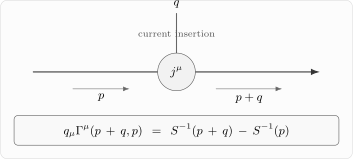
The Ward–Takahashi identity says that contracting the amputated current insertion with its momentum subtracts the reduced inverse propagators on its two sides. Here $S_F=iS$ and the source-rule factor $i$ is removed from $\Gamma^\mu$. This is the diagrammatic form of charge conservation inside correlation functions.

This identity is much stronger than the classical equation $\partial_\mu j^\mu=0$. It constrains loop corrections. In QED it implies, after renormalization, the equality of the vertex and fermion wavefunction renormalization constants in a gauge-invariant scheme. More generally, it is the algebraic reason why gauge invariance organizes counterterms.

Background sources and transverse polarization

A clean way to package Ward identities is to couple a source to the current. We use the vacuum in-out functional with the Feynman boundary prescription: its derivatives generate time-ordered correlators, while retarded response requires a separate continuation and boundary prescription. Write

$$Z[A]=e^{iW[A]} =\int \mathcal D\Phi\, \exp\left(iS_0+i\int d^dx\,A_\mu j^\mu\right).$$

The current expectation value in the background $A$ is

$$\langle j^\mu(x)\rangle_A=+{\delta W[A]\over\delta A_\mu(x)}.$$

If the source $A_\mu$ is interpreted as a background gauge field, then the local transformation

$$\psi(x)\mapsto e^{+i\alpha(x)}\psi(x), \qquad A_\mu(x)\mapsto A_\mu(x)+\partial_\mu\alpha(x)$$

leaves the source-coupled theory invariant. Therefore

$$W[A+\partial\alpha]=W[A].$$

Expanding to first order in $\alpha$ gives

$$0=\int d^dx\,\partial_\mu\alpha(x){\delta W\over\delta A_\mu(x)} =-\int d^dx\,\alpha(x)\partial_\mu{\delta W\over\delta A_\mu(x)}.$$

Since $\alpha(x)$ is arbitrary,

$$\boxed{ \partial_\mu{\delta W[A]\over\delta A_\mu(x)}=0. }$$

Differentiating this identity once more with respect to $A_\nu$ and then setting $A=0$ gives transversality of the current-current correlator,

$$\partial_\mu^x\Pi^{\mu\nu}(x-y)=0,$$

where

$$\Pi^{\mu\nu}(x-y) =i\langle Tj^\mu(x)j^\nu(y)\rangle_{\rm conn} +\text{possible local contact terms}.$$

In momentum space,

$$\boxed{ q_\mu\Pi^{\mu\nu}(q)=0. }$$

Lorentz invariance then fixes the nonlocal parity-even part of the two-point function to have the form

$$\boxed{ \Pi^{\mu\nu}(q) =\left(q^\mu q^\nu-q^2\eta^{\mu\nu}\right)\Pi(q^2) +\text{local transverse terms}. }$$

This formula is familiar from vacuum polarization, but here the lesson is more general: a conserved current can only generate a transverse response. In gauge theory, this is why a photon mass term $A_\mu A^\mu$ is forbidden by gauge invariance, while a correction to $F_{\mu\nu}F^{\mu\nu}$ is allowed.

There is one subtlety that will matter below. The correlator $\langle Tj^\mu j^\nu\rangle$ by itself is not always the whole $\Pi^{\mu\nu}$. Local contact terms can be added by local counterterms in $W[A]$. They do not affect separated-point current conservation, but they do affect the precise Ward identity at coincident points. Gauge invariance often fixes those local terms.

Chiral symmetry of a massless Dirac field

In the $1+1$-dimensional theory used on this page, the massless Dirac Lagrangian has an additional classical symmetry. The matrix $\gamma^5=\gamma^0\gamma^1$ fixed above obeys

$$\{\gamma^5,\gamma^\mu\}=0, \qquad (\gamma^5)^2=1, \qquad (\gamma^5)^\dagger=\gamma^5.$$

In higher even dimensions the corresponding chirality matrix contains a dimension- and signature-dependent phase. In four-dimensional Lorentzian formulas elsewhere on the site it is the inherited $\gamma_5=i\gamma^0\gamma^1\gamma^2\gamma^3$; that convention is not being redefined here.

For $m=0$,

$$\mathcal L_0=\bar\psi i\gamma^\mu\partial_\mu\psi$$

is invariant under the axial rotation

$$\psi\mapsto e^{i\beta\gamma^5}\psi, \qquad \bar\psi\mapsto \bar\psi e^{i\beta\gamma^5}.$$

The corresponding axial current is

$$\boxed{ j_5^\mu=\bar\psi\gamma^\mu\gamma^5\psi. }$$

Classically,

$$\partial_\mu j_5^\mu=0 \qquad (m=0).$$

If the mass is nonzero, the axial symmetry is explicitly broken. A direct variation gives

$$\boxed{ \partial_\mu j_5^\mu=2im\bar\psi\gamma^5\psi }$$

in Minkowski signature. The vector current remains conserved because the mass term preserves ordinary phase rotations.

The chiral projectors

$$P_\pm={1\over2}(1\pm\gamma^5)$$

split the fermion into two eigenspace components. In the propagation-label convention declared above, the full field is

$$\psi=\psi_++\psi_-.$$

The vector and axial rotations are equivalently independent phase rotations of these two components. With the vector convention above, the axial rotation $\psi\mapsto e^{i\beta\gamma^5}\psi$, and $\psi_+=P_-\psi$, $\psi_-=P_+\psi$,

$$\psi_+\mapsto e^{+i\alpha-i\beta}\psi_+, \qquad \psi_-\mapsto e^{+i\alpha+i\beta}\psi_-.$$

The mass term mixes the two chiralities. Schematically,

$$m\bar\psi\psi =m\left(\bar\psi_+\psi_-+\bar\psi_-\psi_+\right),$$

so it is invariant under the vector phase but not under the axial phase. This is the simplest way to remember why a massless fermion has more symmetry than a massive fermion.

For $N$ massless Dirac fermions with identical kinetic terms, the symmetry is enlarged. In four dimensions, at the classical level and with no other flavor-breaking interactions, one has independent flavor rotations of left- and right-handed fermions,

$$U(N)_L\times U(N)_R.$$

To determine what a mass term preserves, work in a basis with positive nonzero masses $M=\operatorname{diag}(m_1,\ldots,m_N)$. For $\psi_L\mapsto U_L\psi_L$ and $\psi_R\mapsto U_R\psi_R$,

$$\begin{aligned} \mathcal L_m&=-\bar\psi_LM\psi_R-\bar\psi_RM\psi_L,\\ \mathcal L_m\ \hbox{invariant} &\quad\Longleftrightarrow\quad U_L^\dagger M U_R=M. \end{aligned}$$

Unitarity then implies $U_LM^2U_L^\dagger=M^2$. Since $M$ is positive, $U_L$ commutes with $M$, and the original equation gives $U_R=U_L=U$. The surviving symmetry is therefore the vector stabilizer $\{U\in U(N):[U,M]=0\}$. Distinct masses leave $U(1)^N$; equal-mass blocks of sizes $n_a$ leave $\prod_a U(n_a)$. Only when all the nonzero masses are equal does the full diagonal $U(N)_V$ survive. For example, a rotation mixing two flavors fails to commute with $\operatorname{diag}(m_1,m_2)$ when $m_1\ne m_2$.

If a block is exactly massless, its left and right rotations remain independent. These are symmetries of the classical Lagrangian; anomalies and a symmetry-breaking vacuum require separate analysis. The two-flavor QCD example and its equal-mass condition are developed in Schwartz 2014, § 28.2.2, pp. 566–567. This approximate chiral flavor symmetry organizes low-energy QCD when quark masses are small compared with the strong scale.

Two-dimensional chiral components

Two dimensions are special because a massless Dirac equation separates into two one-dimensional propagation equations. With the light-cone conventions in the note above, the free massless action can be written as

The labels $+$ and $-$ are convention labels, not universal names for “right” and “left.” What matters physically is the equation of motion: one component propagates along constant $x^-$ and the other along constant $x^+$. When comparing references, translate the light-cone convention before comparing signs in the axial current.

$$S_0=\int d^2x\, \left(2i\psi_+^\dagger\partial_-\psi_+ +2i\psi_-^\dagger\partial_+\psi_-\right).$$

The equations of motion are

$$\boxed{ \partial_-\psi_+=0, \qquad \partial_+\psi_-=0. }$$

Therefore

$$\psi_+=\psi_+(x^+), \qquad \psi_-=\psi_-(x^-)$$

on shell. The two chiral densities are

$$J_+=\psi_+^\dagger\psi_+, \qquad J_-=\psi_-^\dagger\psi_-.$$

For these unrescaled projector components,

$$j^0=J_++J_-, \qquad j^1=-J_++J_-, \qquad A_\mu j^\mu=\widehat A_-J_++\widehat A_+J_-.$$

They obey

$$\partial_-J_+=0, \qquad \partial_+J_-=0$$

classically. The vector and axial currents are the sum and difference of the chiral currents. In the convention $j_5^\mu=-\epsilon^{\mu\nu}j_\nu$, the axial current is not an independent object in two dimensions; it is the Hodge dual of the vector current.

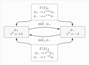
The two chiral components are independent when $m=0$. Here the propagation labels obey $\psi_+=P_-\psi$ and $\psi_-=P_+\psi$, as shown by their $\gamma^5$ eigenvalues. The vector rotation acts with the same phase on both components, while the axial rotation acts with opposite phases. A Dirac mass couples the two chiralities and breaks the axial symmetry.

The free propagator of a chiral component has a characteristic distributional form. With the Cartesian measure and unrescaled fields above,

$$\langle T\psi_+(x)\psi_+^\dagger(0)\rangle ={1\over2\pi i}\,K_+(x), \qquad K_+(x):={1\over x^+-i0\operatorname{sgn}(x^-)}.$$

The pole prescription remembers time ordering. It also hides a contact term. The useful identity is

$${1\over x^+-i0\operatorname{sgn}(x^-)} =\mathcal P{1\over x^+}+i\pi\operatorname{sgn}(x^-)\delta(x^+),$$

so

$$\partial_-{1\over x^+-i0\operatorname{sgn}(x^-)} =2\pi i\,\delta(x^+)\delta(x^-).$$

This is the Lorentzian cousin of

$$\partial_{\bar z}{1\over z}=\pi\delta^{(2)}(z).$$

The lesson is small but important: a chiral propagator looks holomorphic away from coincident points, but its derivative is not zero as a distribution. Contact terms are precisely what make Ward identities true.

The Thirring interaction as an auxiliary vector field

The massless Thirring model is the two-dimensional current-current theory below. Here the written current and current products denote renormalized composites with Coleman’s unit-charge Ward normalization and matched finite current-product prescription; another prescription can redefine the coupling called $g$:

$$\mathcal L_{\rm Th} =\bar\psi i\gamma^\mu\partial_\mu\psi -{g\over2}j_\mu j^\mu, \qquad j^\mu=\bar\psi\gamma^\mu\psi.$$

For normal-ordered products of the unrescaled components defined above,

$$j_\mu j^\mu=4J_+J_-.$$

Therefore the Cartesian-measure component form is exactly

$$\mathcal L_{\rm Th} =2i\psi_+^\dagger\partial_-\psi_+ +2i\psi_-^\dagger\partial_+\psi_- -2gJ_+J_-.$$

The interaction couples the two chiral densities, but it does not mix the fields $\psi_+$ and $\psi_-$ the way a mass term would. It preserves the vector and axial $U(1)$ symmetries. Power counting makes $g$ dimensionless, so the interaction is classically marginal. Symmetry and power counting alone do not prove gaplessness.

The matched bosonic dictionary supplies the additional information. For a compact phase $\Phi$ of period $2\pi$, $j^\mu=\epsilon^{\mu\nu}\partial_\nu\Phi/(2\pi)$ gives $j_\mu j^\mu=-(\partial\Phi)^2/(4\pi^2)$ in the stated Lorentzian signature. Adding the interaction to the free coefficient $1/(8\pi)$ therefore gives the kinetic coefficient $K/(8\pi)$, with $K=1+g/\pi$. A positive scalar Hamiltonian requires $K>0$, or $g>-\pi$. In this prescription and domain the massless one-flavor model is a free compact scalar with a coupling-dependent radius and hence a gapless line of fixed points. Zero stiffness is singular, and negative stiffness is not another unitary point on that line. See Coleman 1975, § I, pp. 2088–2089, Eqs. (1.4)–(1.10), and § IV, p. 2093, Eqs. (4.22)–(4.29). The current normalization and radius change are developed later in the course.

This conclusion is specific to the Abelian one-flavor interaction written above. With several flavors there are inequivalent ways to contract flavor and chiral indices. Non-Abelian current-current or Gross–Neveu interactions can have nonzero beta functions and dynamically generate a scale. The number of flavors by itself is therefore not enough information: the operator and its symmetry representation must also be specified.

For real $g\ne0$, a useful rewriting introduces an auxiliary vector field $A_\mu$ with no kinetic term. Use a common finite regulator and normalize its Lorentzian Gaussian integral by the zero-current value. Define the integral over real components with positive Gaussian damping, removed only after evaluation at fixed regulator:

$$\mathcal L =\bar\psi i\gamma^\mu\partial_\mu\psi +A_\mu j^\mu+{1\over2g}A_\mu A^\mu.$$

The equation of motion for $A_\mu$ is algebraic,

$$A^\mu=-g j^\mu.$$

Substituting back gives

$$+A_\mu j^\mu+{1\over2g}A_\mu A^\mu =-{g\over2}j_\mu j^\mu.$$

Completing the square gives $(A+gj)^2/(2g)-gj^2/2$. At finite damping the Gaussian uses the damped quadratic inverse; removing that damping after evaluation yields the displayed interaction with a current-independent normalization. This regulated identity does not prove continuum existence or a positive Euclidean real-contour representation at every coupling. The free point $g=0$ is treated directly, or as a limit after eliminating $A_\mu$. The figure shows the two equivalent forms under this prescription.

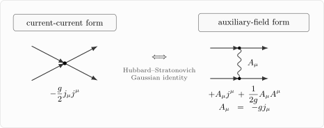
The Hubbard–Stratonovich rewriting uses a common finite regulator and the normalized Lorentzian Gaussian prescription at real $g\ne0$. Completing the square returns the negative current-current interaction shown on the left. Its relative sign is fixed by the displayed source coupling and auxiliary quadratic term; the exchange drawing is schematic.

Integrating out the fermions gives their background functional $W[A]$. The full auxiliary effective action is $\int d^2x\,A_\mu A^\mu/(2g)+W[A]$, where

$$e^{iW[A]}=\int \mathcal D\psi\mathcal D\bar\psi\, \exp\left(i\int d^2x\,\bar\psi i\gamma^\mu(\partial_\mu-iA_\mu)\psi\right),$$

or formally

$$W[A]=-i\operatorname{Tr}\log\left(i\gamma^\mu(\partial_\mu-iA_\mu)\right).$$

Expanding $W[A]$ in powers of $A$ generates time-ordered current correlators. With a regulator and counterterms preserving the vector Ward identity, this fermion functional is gauge invariant as a background functional. The full auxiliary action is not: its $A_\mu A^\mu/(2g)$ term changes under $A_\mu\mapsto A_\mu+\partial_\mu\alpha$, so the auxiliary integral has no ordinary gauge redundancy. The next page computes the quadratic part of $W[A]$ carefully; local counterterms in $W[A]$ decide which Ward identities are preserved.

This last sentence is the practical bridge to anomalies. The separated-point determinant may look symmetric under several classical transformations, but the local terms required to define it can privilege one symmetry over another. For a dynamical gauge field, preserving the gauge symmetry is not optional.

Vector Ward identity versus axial Ward identity

For a massless two-dimensional Dirac fermion, the vector and axial currents are related by

$$j_5^\mu=-\epsilon^{\mu\rho}j_\rho.$$

Define the vector two-point function

$$\Pi^{\mu\nu}(q)=i\int d^2x\,e^{iq\cdot x} \langle Tj^\mu(x)j^\nu(0)\rangle_{\rm conn} +\text{contact terms}.$$

If vector gauge invariance is imposed, then

$$q_\mu\Pi^{\mu\nu}(q)=0.$$

In two dimensions, the one-loop result has the nonlocal structure

$$\Pi^{\mu\nu}(q) ={1\over\pi}\left(\eta^{\mu\nu}-{q^\mu q^\nu\over q^2}\right)$$

for one unit-charge Dirac fermion with the source functional defined above. Its nonlocal sign is fixed by $Z[A]=e^{iW[A]}$ and the coupling $+A_\mu j^\mu$; local counterterms can change polynomial contact terms but cannot reverse this nonlocal projector. The tensor is transverse:

$$q_\mu\Pi^{\mu\nu}(q)=0.$$

Now form the mixed axial-vector correlator

$$\Pi_5^{\mu\nu}(q) =i\int d^2x\,e^{iq\cdot x} \langle Tj_5^\mu(x)j^\nu(0)\rangle_{\rm conn}.$$

Using $j_5^\mu=-\epsilon^{\mu\rho}j_\rho$ gives

$$\Pi_5^{\mu\nu}(q)=-\epsilon^{\mu\rho}\Pi_\rho{}^\nu(q).$$

Therefore

$$q_\mu\Pi_5^{\mu\nu}(q) =-q_\mu\epsilon^{\mu\rho}{1\over\pi} \left(\delta_\rho{}^\nu-{q_\rho q^\nu\over q^2}\right).$$

The second term vanishes because $q_\mu\epsilon^{\mu\rho}q_\rho=0$. Hence

$$\boxed{ q_\mu\Pi_5^{\mu\nu}(q) ={1\over\pi}\epsilon^{\nu\rho}q_\rho. }$$

Because the vector source enters as $+A_\nu j^\nu$, the linear variation of this time-ordered generating functional gives $\langle j_5^\mu\rangle_A=+\Pi_5^{\mu\nu}A_\nu+O(A^2)$. Thus, suppressing the Fourier factor of $i$,

$$q_\mu\langle j_5^\mu\rangle_A =+{1\over\pi}\epsilon^{\nu\rho}q_\rho A_\nu =-{1\over\pi}\epsilon^{\rho\nu}q_\rho A_\nu.$$

In position space this is the axial anomaly in a background gauge field:

$$\boxed{ \partial_\mu\langle j_5^\mu\rangle_A =-{1\over\pi}\epsilon^{\mu\nu}\partial_\mu A_\nu =-{1\over2\pi}\epsilon^{\mu\nu}F_{\mu\nu}. }$$

Thus the vector current can be conserved, or the axial current can be conserved, but not both in a gauge-invariant quantum theory with a background vector field. For a dynamical gauge field, preserving vector gauge invariance is mandatory; the axial symmetry becomes anomalous.

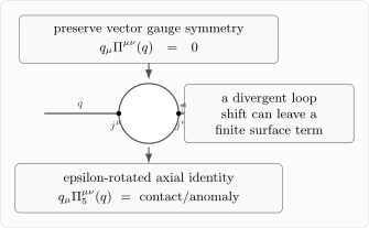
The same current-current loop tests both vector and axial Ward identities in two dimensions. A gauge-invariant choice of local counterterms preserves $q_\mu\Pi^{\mu\nu}=0$ and leaves a finite contact term in the epsilon-rotated axial identity.

There is a useful diagrammatic way to see why a contradiction can occur. Contracting the vacuum polarization graph with $q_\mu$ gives

$$q_\mu\Pi^{\mu\nu}(q) \sim \int {d^dp\over(2\pi)^d}\, \operatorname{tr}\left[ \gamma^\nu S(p+q)q\!\!\!/ S(p) \right].$$

At this one-loop step $S$ is the free reduced propagator. Since

$$q\!\!\!/=S^{-1}(p+q)-S^{-1}(p),$$

one is tempted to write

$$q_\mu\Pi^{\mu\nu}(q) \sim \int {d^dp\over(2\pi)^d}\, \operatorname{tr}\,\gamma^\nu\left[S(p)-S(p+q)\right] =0$$

by shifting the integration variable. This argument is legitimate only if the integral is sufficiently convergent or if the regulator respects the shift. In anomalous diagrams, the formal shift changes the boundary of the regulated integration region. A finite surface term can survive.

A one-dimensional caricature is

$$\int_{-\Lambda}^{\Lambda}dp\,[f(p+q)-f(p)] \simeq q\int_{-\Lambda}^{\Lambda}dp\,f'(p) =q[f(\Lambda)-f(-\Lambda)].$$

If the boundary term remains finite as $\Lambda\to\infty$, the naive shift fails. The anomaly is a regulated version of precisely this phenomenon.

Summary

A continuous symmetry gives a current. In a quantum field theory, the corresponding conservation law becomes a Ward identity: the divergence of the current inside a correlation function is zero away from insertions, but has contact terms at coincident points. In momentum space, the vector Ward identity for a fermion current is

$$q_\mu\Gamma^\mu(p+q,p)=S^{-1}(p+q)-S^{-1}(p).$$

Coupling the current to a background field turns the same statement into gauge invariance of $W[A]$. Differentiating gauge invariance gives transversality of current correlators,

$$q_\mu\Pi^{\mu\nu}(q)=0.$$

Massless fermions have chiral symmetries. In two dimensions, the massless Dirac fermion splits into independent chiral components $\psi_+(x^+)$ and $\psi_-(x^-)$. The Thirring interaction couples their densities but does not create a mass term, so it preserves the vector and axial $U(1)$ symmetries. With the matched current prescription, its massless fixed line has positive stiffness for $g>-\pi$; gaplessness follows from the bosonic solution, not from symmetry and power counting alone.

The quantum theory adds the crucial caveat: not every classical symmetry survives regularization. In two dimensions, preserving vector gauge invariance forces the axial current to satisfy

$$\partial_\mu j_5^\mu=-{1\over2\pi}\epsilon^{\mu\nu}F_{\mu\nu}$$

for one unit-charge massless Dirac fermion. This is the first anomaly in the course. Notice the logic: the anomaly is not a failure of algebra at separated points; it is a statement about the regulated contact terms of composite currents. The next page studies those current-current correlators and local counterterms more explicitly.

Common pitfalls

Replacing a Ward identity by $\partial_\mu j^\mu=0$. Inside time-ordered products, contact terms are part of the statement and generate the symmetry action on coincident insertions.

Demanding both vector and axial conservation after regularization. The two currents can coexist classically, but a regulator may not preserve both. In a gauge theory, vector gauge invariance is the identity that must be preserved.

Treating $j_5^\mu=-\epsilon^{\mu\nu}j_\nu$ as equality of Ward identities. The identity means that the same correlator is tested in two different tensor directions. A transverse vector correlator generally has an anomalous axial divergence.

Calling a current-current interaction a mass term. In the matched prescription and positive-stiffness domain, the Thirring coupling changes the radius along a massless fixed line. The mass term $\bar\psi\psi$ mixes chiralities and breaks axial symmetry; it is relevant at the free point, but its scaling dimension changes along the interacting line. Massless kinetic positivity alone does not determine the fate of this perturbation.

Exercises

Exercise 1: Derive the contact-term Ward identity

Let a field $\Phi_k$ have charge $Q_k$ under the global $U(1)$ convention used on this page, so that

$$\delta\Phi_k=+i\alpha Q_k\Phi_k.$$

Use a smooth compactly supported local parameter $\alpha(x)$ and the symmetry-preserving regulated integration data assumed above to derive the Ward identity for

$$\left\langle Tj^\mu(x)\Phi_1(x_1)\cdots\Phi_n(x_n)\right\rangle.$$

Solution

Under a local transformation, the action changes by

$$\delta S=-\int d^dx\,\partial_\mu\alpha(x)j^\mu(x) =+\int d^dx\,\alpha(x)\partial_\mu j^\mu(x).$$

The path integral is invariant under a change of variables:

$$0=\left\langle i\delta S\,T\Phi_1\cdots\Phi_n\right\rangle +\left\langle T\delta(\Phi_1\cdots\Phi_n)\right\rangle.$$

The operator variation is

$$\delta(\Phi_1\cdots\Phi_n) =+i\sum_{k=1}^n\alpha(x_k)Q_k\Phi_1\cdots\Phi_k\cdots\Phi_n.$$

Writing $\alpha(x_k)=\int d^dx\,\alpha(x)\delta^{(d)}(x-x_k)$ and using the arbitrariness of $\alpha(x)$ gives

$$\boxed{ \begin{aligned} &\partial_\mu^x\left\langle Tj^\mu(x)\prod_{\ell=1}^n\Phi_\ell(x_\ell) \right\rangle \\ &\qquad=-\sum_{k=1}^n Q_k\delta^{(d)}(x-x_k) \left\langle T\prod_{\ell=1}^n\Phi_\ell(x_\ell)\right\rangle \end{aligned} }.$$

Both terms in the change-of-variables equation carry $+i$ before their common factor is divided out. Moving the insertion variation to the other side produces the minus sign in the contact identity. For $\psi$ and $\bar\psi$, the charges $+1$ and $-1$ reproduce the two-point identity in the main text. The divergence is supported only at the operator insertions.

Exercise 2: Construct the transverse current tensor

Assume Lorentz invariance and current conservation in a parity-even theory. Show that a two-point function of conserved currents in momentum space has the form

$$\Pi^{\mu\nu}(q)=\left(q^\mu q^\nu-q^2\eta^{\mu\nu}\right)\Pi(q^2)$$

up to local transverse terms.

Solution

The most general parity-even rank-two tensor built from $q^\mu$ and $\eta^{\mu\nu}$ is

$$\Pi^{\mu\nu}(q)=A(q^2)\eta^{\mu\nu}+B(q^2)q^\mu q^\nu.$$

Current conservation gives

$$0=q_\mu\Pi^{\mu\nu}(q) =A(q^2)q^\nu+B(q^2)q^2q^\nu.$$

For generic $q$, this requires

$$A(q^2)=-q^2B(q^2).$$

Therefore

$$\Pi^{\mu\nu}(q)=B(q^2)\left(q^\mu q^\nu-q^2\eta^{\mu\nu}\right).$$

Renaming $B(q^2)=\Pi(q^2)$ gives the stated form. Polynomial transverse pieces correspond to local gauge-invariant counterterms.

Exercise 3: Derive the axial anomaly from vector response

In two dimensions, suppose the vector current correlator of one massless Dirac fermion is

$$\Pi^{\mu\nu}(q)={1\over\pi} \left(\eta^{\mu\nu}-{q^\mu q^\nu\over q^2}\right).$$

Using $j_5^\mu=-\epsilon^{\mu\rho}j_\rho$, compute $q_\mu\Pi_5^{\mu\nu}(q)$.

Solution

The mixed axial-vector correlator is

$$\Pi_5^{\mu\nu}(q)=-\epsilon^{\mu\rho}\Pi_\rho{}^\nu(q).$$

Thus

$$q_\mu\Pi_5^{\mu\nu}(q) =-{1\over\pi}q_\mu\epsilon^{\mu\rho} \left(\delta_\rho{}^\nu-{q_\rho q^\nu\over q^2}\right).$$

The second term vanishes because

$$q_\mu\epsilon^{\mu\rho}q_\rho=0.$$

Therefore

$$q_\mu\Pi_5^{\mu\nu}(q) =-{1\over\pi}q_\mu\epsilon^{\mu\nu}.$$

Since $q_\mu\epsilon^{\mu\nu}=-\epsilon^{\nu\rho}q_\rho$, we find

$$\boxed{ q_\mu\Pi_5^{\mu\nu}(q)={1\over\pi}\epsilon^{\nu\rho}q_\rho. }$$

This is the momentum-space axial anomaly in the convention used on this page.

Exercise 4: Integrate out the Thirring auxiliary field

For real $g\ne0$, use the common finite regulator and normalized Lorentzian Gaussian prescription specified above to show that integrating out the auxiliary field in

$$\mathcal L_A=\bar\psi i\gamma^\mu\partial_\mu\psi +A_\mu j^\mu+{1\over2g}A_\mu A^\mu$$

reproduces the Thirring interaction $-(g/2)j_\mu j^\mu$.

Solution

The $A_\mu$ equation of motion is

$$+j^\mu+{1\over g}A^\mu=0,$$

so

$$A^\mu=-gj^\mu.$$

Substitute this into the $A$-dependent part of the Lagrangian:

$$+A_\mu j^\mu+{1\over2g}A_\mu A^\mu =-g j_\mu j^\mu+{1\over2g}g^2j_\mu j^\mu.$$

Hence

$$+A_\mu j^\mu+{1\over2g}A_\mu A^\mu =-{g\over2}j_\mu j^\mu.$$

The auxiliary-field path integral gives the same result, up to an irrelevant Gaussian normalization.

Exercise 5: Expose the chiral propagator contact term

For the normalized singular kernel of the massless two-dimensional chiral propagator,

$$K_+(x)={1\over x^+-i0\operatorname{sgn}(x^-)},$$

use

$${1\over x^+-i0\operatorname{sgn}(x^-)} =\mathcal P{1\over x^+}+i\pi\operatorname{sgn}(x^-)\delta(x^+)$$

to show that $\partial_-K_+(x)$ is a contact term.

Solution

The principal-value term has no $x^-$ dependence, so

$$\partial_-\mathcal P{1\over x^+}=0.$$

The second term gives

$$\partial_-\left(i\pi\operatorname{sgn}(x^-)\delta(x^+)\right) =i\pi\left(2\delta(x^-)\right)\delta(x^+).$$

Therefore

$$\boxed{ \partial_-K_+(x)=2\pi i\,\delta(x^+)\delta(x^-). }$$

Thus the chiral propagator kernel is annihilated by $\partial_-$ away from the origin, but not as a distribution. This is exactly the kind of contact term that appears in Ward identities.

References

• S. Coleman, “Quantum sine-Gordon equation as the massive Thirring model”, Physical Review D 11 (1975) 2088–2097.
• D. J. Gross and A. Neveu, “Dynamical Symmetry Breaking in Asymptotically Free Field Theories”, Physical Review D 10 (1974) 3235–3253.
• Schwartz, Matthew D. Quantum Field Theory and the Standard Model. Cambridge University Press (2014). DOI.
• Y. Takahashi, “On the Generalized Ward Identity”, Il Nuovo Cimento 6 (1957) 371–375.
• W. E. Thirring, “A Soluble Relativistic Field Theory”, Annals of Physics 3 (1958) 91–112.
• J. C. Ward, “An Identity in Quantum Electrodynamics”, Physical Review 78 (1950) 182.

Further reading

• S. Coleman, Lectures of Sidney Coleman on Quantum Field Theory, B. Gin-ge Chen, D. Derbes, D. Griffiths, B. Hill, R. Sohn, and Y.-S. Ting (eds.), World Scientific (2019), especially the lectures on symmetries, Ward identities, and two-dimensional fermions.
• A. M. Polyakov, Gauge Fields and Strings, Harwood Academic Publishers (1987), especially the discussions of two-dimensional field theory and anomalies.
• M. Srednicki, Quantum Field Theory, Cambridge University Press (2007), sections on continuous symmetries, Ward identities, and anomalies.
• S. Weinberg, The Quantum Theory of Fields, Vols. I–II, Cambridge University Press (1995–1996), chapters on symmetries, current algebra, and anomalies.
• A. Zee, Quantum Field Theory in a Nutshell, 2nd ed., Princeton University Press (2010), discussions of chiral symmetry, bosonization, and anomalies.