

Schwinger Model and Gauge-Invariant Correlators
The previous page solved a massless two-dimensional fermion in a fixed Abelian background gauge field. The result was almost embarrassingly simple: a chiral propagator is the free chiral propagator multiplied by endpoint phases. That simplicity is deceptive in the best possible way. Once the gauge field is dynamical, those endpoint phases must be averaged over, and the answer depends crucially on gauge invariance.
This page studies the cleanest example: massless QED in two spacetime dimensions, usually called the Schwinger model. It is a small theory with a ridiculous amount of physics packed inside it. There are no transverse photons in dimensions, but the fermion determinant gives the gauge-invariant electric field a massive propagator. Charged fermion two-point functions are not gauge-invariant objects, but Wilson-line dressed correlators are. The same determinant and phase factors also lead naturally to the Cauchy determinants and vertex-operator formulas that become bosonization on the next page.
Required background. Gauge fields in two dimensions supplies the exact background-field propagator, the distinction between open lines and closed-loop determinants, and the light-cone decomposition used here. Helpful background. Ward identities and chiral symmetries supplies the vector Ward identity and axial anomaly, while current correlators and polarization tensors supplies the response-function viewpoint.
QED₂ and the absence of a transverse photon
Section titled “QED₂ and the absence of a transverse photon”Conventions and normalization. This page mostly uses Euclidean functional integrals. The gauge coupling is placed in the Maxwell term rather than in the covariant derivative:
Thus a unit-charge field transforms as
The Euclidean gamma matrices obey
In two dimensions
With these conventions the Schwinger mass for one massless Dirac fermion is
If instead one writes with a canonically normalized gauge field , then and the same physical mass is obtained.
Local formulas and global sectors. The determinant formulas below are for the Euclidean plane, or equivalently for the nonzero modes in the trivial flux sector. On a compact surface, harmonic gauge fields, spin structure, quantized flux, and fermion zero modes add global dependence. They do not change the local polarization tensor or the Schwinger mass .
The Euclidean Schwinger model is
The important starting point is not the determinant, but the kinematics. In four spacetime dimensions a massless gauge field has two transverse polarizations. In dimensions there is no transverse spatial direction. The gauge field still has components , but gauge redundancy and Gauss’ law remove local photon oscillators. The gauge-invariant field strength has one independent component, the electric field.
This is why the Schwinger model should not be described as “the photon eats a scalar” in the Higgs sense. There is no elementary scalar field with a vacuum expectation value. Instead, the fermion loop changes the correlator of the gauge-invariant electric field. A theory with no transverse photon becomes equivalent, in its gauge-invariant sector, to a massive scalar excitation.
The mass dimension also already hints at special behavior. In two dimensions,
The gauge coupling is itself a mass scale. There is no need for dimensional transmutation here; the scale is present from the beginning. What is nontrivial is that this scale appears as a gauge-invariant pole in correlation functions.
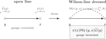
An open charged fermion propagator is gauge covariant, not gauge invariant. A Wilson-line dressing supplies the missing endpoint phase and produces a gauge-invariant charged-pair operator.
Integrating out the fermion
Section titled “Integrating out the fermion”For a fixed background , the fermion integral is Gaussian:
where
Define the effective action by
For one massless Dirac fermion, gauge-invariant regularization gives the exact Abelian result
Equivalently,
The second form is often the more physical one. It says that the determinant depends only on the gauge-invariant electric field, not on the pure-gauge part of . The nonlocal operator is the two-dimensional Coulomb Green function. Thus a massless fermion loop turns a local Maxwell theory into a theory with a nonlocal electric-field term.
In momentum space, let
Then
The tensor is transverse:
This transversality is the momentum-space form of vector gauge invariance. A regulator that spoils it has changed the theory.
Why the determinant stops at quadratic order
Section titled “Why the determinant stops at quadratic order”The word “exact” deserves an explanation. Expanding the logarithm of the determinant in powers of generates connected correlation functions of the free vector current:
Here the sign follows from the Euclidean coupling used above. For a massless Abelian Dirac fermion in two dimensions, the current algebra is Gaussian: the current can be represented as a derivative of a free scalar. Its connected correlators vanish for . The one-point function vanishes, and the two-point function is the transverse polarization tensor . Consequently, all local nonzero-mode dependence of the determinant is already contained in the quadratic term.
This truncation is special. A fermion determinant is always a one-loop object, but in a generic theory that one loop has nonzero vertices with arbitrarily many external gauge fields. Non-Abelian currents, fermion masses, and global holonomy sectors invalidate the simple Gaussian argument.
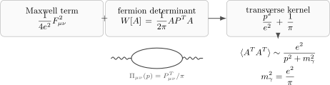
The massless fermion loop produces a transverse quadratic term . Combined with the Maxwell action, the transverse gauge field has denominator with .
The Schwinger mass
Section titled “The Schwinger mass”The total effective action for the gauge field is
Since only the transverse part of is physical, write with
The Maxwell term is
and the determinant is
Therefore
The transverse gauge-field propagator is proportional to
Thus the gauge-invariant mass scale is
The field strength has the Euclidean two-point function
The numerator is not a mistake. Since is a derivative of , its two-point function contains a contact term. Indeed,
At separated points, the contact term drops out and the remaining correlation decays with mass . This is the precise sense in which the Schwinger model has a massive gauge-invariant excitation.
There is a useful real-time derivation of the same mass. In Minkowski signature, the vector current is conserved, while the axial current has the anomaly
in the unit-charge convention above. With , the vector and axial currents are dual:
The minus sign is fixed here by , the mostly-minus metric, and ; changing any of those conventions requires translating both this identity and the anomaly together. Combining this relation with Maxwell’s equation gives
This derivation is less useful for computing all correlators, but it makes the physics vivid: the anomaly turns the electric field into a massive propagating scalar.
What is massive in the Schwinger model?
Section titled “What is massive in the Schwinger model?”The phrase “the photon becomes massive” is useful but slightly dangerous in dimensions. There was no transverse photon oscillator to begin with. The gauge-invariant statement is that the electric-field correlator has a massive pole. To distinguish the two signatures, write and in the site’s -dimensional Lorentzian extension. The Feynman continuation is
Thus the physical Lorentzian pole is
The equation instead locates the pole of the analytically continued Euclidean denominator; it is not a pole at real Euclidean momentum. This agrees with the signed Lorentzian polarization and Maxwell kernel and the canonical massive-scalar equation. In Euclidean language the separated-point part of
is governed by the denominator . The first term is a contact term. It matters for Ward identities and short-distance normalization, but it does not produce a long-distance force. Continuing the full electric-field correlator also continues its tensor components and contact prescription; the negative separated-point Euclidean term is not a negative-norm Lorentzian state.
This distinction is helpful when comparing QED₂ with the Higgs mechanism. The Schwinger mass is generated by vacuum polarization and the anomaly; it is not a local gauge-noninvariant Proca term.
Screening of external charges
Section titled “Screening of external charges”Pure electrodynamics in one spatial dimension confines external charges linearly. Put charges and a distance apart, with measured in units of the dynamical fermion charge. Gauss’ law forces a constant electric field between them, so the energy grows like
In the massless Schwinger model the fermion determinant modifies the static gauge propagator. In a convenient gauge, the static kernel is
Therefore the interaction energy of the two opposite external charges is
Using
we get
At small separation, this reduces to the pure one-dimensional Coulomb result:
At large separation, it saturates:
The massless dynamical fermions screen external charges. This is why one must be careful with the word “confinement” in two-dimensional gauge theory. Pure QED₂ has a linear potential, whereas the massless Schwinger model screens. Massive matter adds pair-production thresholds and charge-lattice effects rather than a single universal interpolation; the later confinement-and-screening lesson treats those distinctions.
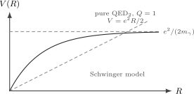
In pure QED₂, the static potential between opposite external charges grows linearly. In the massless Schwinger model, vacuum polarization gives the gauge field the Schwinger mass and the potential saturates at large separation.
Open fermion propagators are gauge covariant
Section titled “Open fermion propagators are gauge covariant”Now consider the fermion Green function in a fixed background:
Under a gauge transformation,
as an operator acting on charge-one fields. Therefore the inverse transforms as
This is exactly the transformation law of the operator product . It is covariant, not invariant.
Suppose we try to define the gauge-field averaged open propagator without gauge fixing:
Strictly speaking, both the numerator and denominator contain the infinite gauge-orbit volume. One can regulate the theory, divide by that common volume, and then use gauge invariance to project insertions onto the invariant sector. Changing variables gives
The function is arbitrary. Unless , the only gauge-invariant answer is
This is the local gauge-theory version of a simple warning: a charged field is not an observable. One may compute a charged propagator after choosing a gauge, but then the answer is a gauge-dependent diagnostic, not a gauge-invariant correlation function. The same distinction appears in gravity: coordinate components may transform covariantly, while an observable must also specify how its insertion points are identified.
This statement is sometimes called Elitzur’s theorem in lattice language. In continuum perturbation theory it is often hidden because gauge fixing is introduced early. The Schwinger model is a good place to keep it visible.
Wilson-line dressed fermion correlators
Section titled “Wilson-line dressed fermion correlators”To build a gauge-invariant charged-pair correlator, connect the two charged insertions by a Wilson line. For a path from to , define
Under ,
Therefore
is gauge invariant:
After integrating out the fermions, the dressed two-point function becomes
This formula separates three pieces of physics:
- is the propagation of a fermion in a fixed background.
- includes the Maxwell action and all closed fermion loops.
- The Wilson line supplies the electric dressing required by gauge invariance.
For a pure gauge field , the fixed-background propagator has the endpoint form
while
The phases cancel, and the dressed object reduces to the free propagator. For a field with nonzero curvature, the answer depends on the path . Different paths differ by a Wilson loop around the area between them. In two-dimensional gauge theory that area is not a minor detail; it measures electric flux.
The path dependence has a simple physical interpretation. A gauge-invariant charged-pair operator does not create a naked fermion and antifermion. It creates them together with a chosen electric string connecting them. The Schwinger mass then determines how that string is screened by the dynamical fermions.
This bilocal operator is neutral as a whole; it does not establish the existence of an isolated charged asymptotic particle. The physical spectrum of the one-flavor massless Schwinger model contains a neutral massive boson. Different dressings can have different overlaps with that spectrum and different short-distance or perimeter contributions.
Gauge-fixed charged propagators and anomalous powers
Section titled “Gauge-fixed charged propagators and anomalous powers”Although open charged propagators are not gauge-invariant observables, they are still useful inside a fixed gauge or in closely related auxiliary-field problems such as the Thirring model. The endpoint phase formula makes their structure transparent.
For one chirality in light-cone coordinates, if
then
A Gaussian average of the phase gives
If the phase field has a logarithmic two-point function,
then
Thus the charged propagator acquires an anomalous power:
This is the mechanism behind the anomalous dimensions in two-dimensional fermion models. The exponent of an open propagator is gauge- and prescription-dependent; it is not by itself a physical scaling dimension. In the Schwinger model, connected correlators of local gauge-invariant operators cluster exponentially because the gauge-invariant spectrum is gapped. The phase-factor calculation is still the bridge to bosonization: a fermion behaves like an exponential of a scalar whose two-point function is logarithmic.
Neutral correlators and the determinant structure
Section titled “Neutral correlators and the determinant structure”Gauge-invariant local operators must be neutral. Examples include the vector current
and scalar or pseudoscalar bilinears such as
When charged fields are brought to the same point to define such bilinears, a short Wilson line should be included before taking the limit. This point-splitting prescription is the gauge-invariant way to define composite operators.
Even before the gauge field is integrated over, free chiral fermions already contain the algebraic pattern that will become bosonization. In this algebraic comparison, use a free complex chiral field with the conformal normalization
For the action-normalized chiral component with propagator , this means . A -point function of therefore carries the additional factor . These are distinct insertion points on the plane, with a fixed radial ordering and consistent continuation of the coordinate differences; this free-field calculation is not the full gauge-averaged Schwinger correlator.
Keep the daggered fields in the literal ascending order shown below. Fermionic Wick contractions then give
Reversing the daggered block takes fermionic interchanges. The reversed order gives the positive determinant. The signs come from these actual interchanges, as required for fermionic ordered products Schwartz 2014, §12.4, p. 212. For example, the direct pairing of crosses one field and is negative; the exchange pairing crosses two and is positive:
The determinant itself still has its usual direct-minus-exchange form,
The general Cauchy determinant is
This formula is identical in structure to a correlator of vertex operators of a free scalar with
Indeed,
Here the exponentials are normal ordered. Replacing every in the Cauchy determinant by contributes exactly . The vertex product therefore has the coordinate dependence of the ascending-dagger correlator written above, including its sign; it is not the positive determinant for that same ordering. The proportionality leaves the chosen short-distance normalization explicit. For example, a cutoff-normalized vertex with two-point function must be multiplied by to represent . The corresponding action-normalized fermion carries Tong 2018, §§7.5.2–7.5.3, pp. 371–373, PDF. Full operator identifications additionally specify their branch, zero-mode and Klein-factor prescriptions; the next page develops that dictionary.
The word neutral is an actual selection rule, not merely a convenient choice of examples. For normal-ordered vertex operators
split the scalar into its constant mode and its fluctuating part,
The constant-mode integral contains
so a noncompact boson gives a delta function imposing ; a compact boson gives the corresponding discrete charge-selection rule. Once neutrality holds, the fluctuating Gaussian integral gives
Without neutrality the massless scalar zero mode makes the correlator vanish or leaves it infrared-regulator dependent. Equal numbers of and in this free-fermion correlator are the same selection rule in fermionic language. In the figure, compare the number of fermionic interchanges required by each pairing for the explicit ascending order.
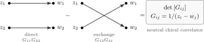
For the free chiral product , Wick’s theorem gives , with . Reversing the two daggered fields gives . The arrows show contractions, not spatial propagation or time evolution; the diagram is schematic.
Summary
Section titled “Summary”The Schwinger model is exactly solvable because several special two-dimensional facts meet at once. A gauge field has no transverse photon polarization. A massless Dirac fermion splits into chiral components. On the plane, the nonzero-mode part of the Abelian fermion determinant is exactly quadratic and gauge invariant. Combining that determinant with the Maxwell term gives a massive gauge-invariant field-strength correlator with
The model also teaches a sharp lesson about observables. The open fermion propagator is gauge covariant, so its gauge-field average vanishes unless a gauge is fixed. A physical charged-pair correlator must include a Wilson-line dressing. Local fermion bilinears and currents are neutral and can be defined gauge invariantly, often by point splitting with a short Wilson line.
Finally, neutral free chiral correlators are determinants multiplied by the parity of the written fermion ordering. Cauchy’s identity then has the product structure of consistently ordered free-boson vertex operators. The scalar zero mode enforces the same neutrality condition as equal fermion and antifermion number. That observation is the doorway to bosonization, the sine-Gordon/Thirring relation, and the two-dimensional confinement/screening comparisons that follow.
Common pitfalls
Section titled “Common pitfalls”Calling the Schwinger mass a Proca term. The mass is not inserted by hand: would violate gauge invariance. The exact determinant produces the transverse structure , or equivalently .
Treating an open propagator as an observable. The ordinary fermion two-point function is not gauge invariant. It can be useful after gauge fixing, but a gauge-invariant charged-pair correlator needs a Wilson line or another dressing, and the result depends on that dressing.
Reading “no photon” as “no gauge dynamics.” The statement means no transverse photon oscillator. The electric field, holonomies, Wilson loops, and response to sources remain meaningful, and the anomaly produces a neutral massive excitation.
Dropping the field-strength contact term. The massive long-distance physics is read from the pole or from separated-point correlators, but the full momentum-space numerator also contains a contact term needed by short-distance identities.
Confusing the determinant with a fixed ordered product. Ascending dagger order contributes relative to the determinant. For , the correlator is exchange minus direct; changing the order changes its sign.
Applying the plane determinant to every global sector. On a compact surface, flux, holonomy, spin structure, and zero modes add information beyond . The local polarization tensor and Schwinger mass remain valid.
Ignoring the scalar neutrality condition. A massless scalar has a constant mode. Vertex-operator correlators are nonzero and infrared finite only when the total vertex charge vanishes.
Exercises
Section titled “Exercises”Exercise 1: Prove Wilson-line dressing is gauge invariant
Section titled “Exercise 1: Prove Wilson-line dressing is gauge invariant”Show that the Wilson-line dressed operator
is gauge invariant under
Solution
The Wilson line transforms as
The fermion factors transform as
Multiplying the phases gives
So the dressed operator is gauge invariant.
Exercise 2: Derive the Schwinger mass and field-strength correlator
Section titled “Exercise 2: Derive the Schwinger mass and field-strength correlator”Starting from
derive the Schwinger mass and the field-strength two-point function
Solution
The transverse gauge-field kernel is
Therefore the transverse propagator is
The pole occurs at
for analytically continued Euclidean momentum. For real Euclidean , this positive kernel has no zero. Under , the denominator becomes , so its Lorentzian pole is at . The physical mass is
In two dimensions, the field strength is one derivative of the transverse gauge field. In momentum space,
inside the transverse subspace. Thus
Exercise 3: Derive the screened static potential
Section titled “Exercise 3: Derive the screened static potential”Evaluate
and show that it tends to a constant as .
Solution
Use the standard integral
The term with gives
The cosine term is the real part of the exponential integral:
Therefore
As , the exponential vanishes and
Thus the potential is screened.
Exercise 4: Keep the sign of the ordered fermion correlator
Section titled “Exercise 4: Keep the sign of the ordered fermion correlator”Use Wick’s theorem to show that
Assume the free chiral propagator is
Solution
There are two nonzero contractions. The direct contraction pairs
Moving past gives one minus sign, so this contribution is
The exchange contraction pairs
Pairing the first field with moves that daggered field past two fields. The two signs cancel, leaving
Adding the two terms gives the stated expression, which is minus the determinant:
As a finite-mode check, for two independent canonical fermion modes. Their contraction matrix is the identity, whose determinant is . Reversing the two creation operators reverses the correlator’s sign.
Exercise 5: Enforce vertex-operator neutrality
Section titled “Exercise 5: Enforce vertex-operator neutrality”Let be a free chiral scalar with
For , show that integration over enforces and that, when this condition holds,
Use at each and at each to recover the product structure of the Cauchy determinant.
Solution
The constant mode factors out:
Therefore
for a noncompact scalar. Thus the correlator vanishes unless the total charge is zero.
For the fluctuating field, the Gaussian identity and normal ordering remove the self-contractions:
Since the two-point function is ,
For charges at and at , the – and – pairs appear in the numerator, while every – pair appears in the denominator:
There are factors in the numerator. Since , this product is times the Cauchy determinant. It matches the ascending-dagger correlator in Exercise4 and the general formula above, with the same short-distance normalization. It would match a positive determinant only after reversing the daggered block and making the corresponding change of vertex ordering.
References
Section titled “References”- S. Coleman, “More About the Massive Schwinger Model,” Annals of Physics 101 (1976), 239–267, doi:10.1016/0003-4916(76)90280-3.
- M. D. Schwartz, Quantum Field Theory and the Standard Model (Cambridge University Press, 2014), doi:10.1017/9781139540940.
- J. Schwinger, “Gauge Invariance and Mass. II,” Physical Review 128 (1962), 2425–2429, doi:10.1103/PhysRev.128.2425.
- D. Tong, Gauge Theory (University of Cambridge lecture notes, 2018), author’s notes, Open PDF, chapter7.
Further reading
Section titled “Further reading”- S. Coleman, Lectures of Sidney Coleman on Quantum Field Theory, edited by B.-G. Chen et al. (World Scientific, 2018).
- A. M. Polyakov, Gauge Fields and Strings (Harwood Academic Publishers, 1987).
- A. Zee, Quantum Field Theory in a Nutshell, 2nd ed. (Princeton University Press, 2010).
- J. Zinn-Justin, Quantum Field Theory and Critical Phenomena, 5th ed. (Oxford University Press, 2021).
Original QFT.org content:CC BY 4.0, unless an item supplies different terms. Third-party material retains its own terms.