Euclidean Continuation and Gaussian Path Integrals

Scattering theory forced us to take the analytic structure of Green functions seriously. Poles identify stable particles, cuts identify multiparticle thresholds, and the $i0$ prescription tells us how to pass around singularities. This page uses the same analytic information in a different direction: it rotates time into the imaginary axis.

The reward is enormous. The Lorentzian path integral

$$\int \mathcal D\phi\,e^{iS[\phi]}$$

is an oscillatory object; it is powerful but not obviously convergent. After Wick rotation, the same free scalar theory is described by a Euclidean functional integral

$$\int \mathcal D\phi\,e^{-S_E[\phi]},$$

which looks like an ordinary Boltzmann weight. This is the first step in the bridge between quantum field theory, classical statistical mechanics, critical phenomena, and finite-temperature field theory.

From oscillatory phases to damping

Wick-rotation convention

On this page the Lorentzian time is rotated as

$$t=-i\tau,$$

so $dt=-i\,d\tau$. With the mostly-minus metric, a scalar action of the form

$$S=\int dt\,d^3x\left[\frac12(\partial_t\phi)^2-\frac12(\nabla\phi)^2-\frac12m^2\phi^2-V_{\mathrm{int}}(\phi)\right]$$

becomes

$$iS=-S_E,$$

where

$$S_E=\int d\tau\,d^3x\left[\frac12(\partial_\tau\phi)^2+\frac12(\nabla\phi)^2+\frac12m^2\phi^2+V_{\mathrm{int}}(\phi)\right].$$

The rotation direction is not a harmless convention by itself. It is tied to the Feynman $i0$ prescription and to the damping of positive-energy states at positive Euclidean time.

Start with the Lorentzian time-ordered correlator of a scalar field,

$$G_F(x_1,\ldots,x_n) =\langle0|T\phi(x_1)\cdots\phi(x_n)|0\rangle.$$

For real times, its path-integral representation is schematically

$$G_F(x_1,\ldots,x_n) ={1\over Z}\int \mathcal D\phi\,e^{iS[\phi]}\phi(x_1)\cdots\phi(x_n).$$

The integrand has modulus one when $S$ is real, so the integral is defined by oscillatory cancellation and by the $i0$ prescription. Euclidean continuation replaces this by a damped integral. For ordered times, insert complete sets of energy eigenstates between the operators. A typical factor is

$$e^{-iE(t_1-t_2)}.$$

If $t=-i\tau$ and $\tau_1>\tau_2$, then

$$e^{-iE(t_1-t_2)}=e^{-E(\tau_1-\tau_2)}.$$

The positive spectrum of the Hamiltonian becomes exponential damping. This is the physical reason Euclidean correlators are better-behaved objects: high-energy intermediate states are suppressed at large Euclidean time separation.

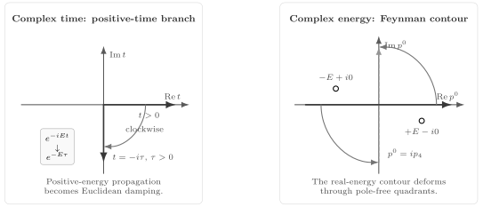
Two related analytic statements must not be conflated. In the complex time plane, the positive-time ordered branch continues as $t=-i\tau$, turning $e^{-iEt}$ into $e^{-E\tau}$. In the complex energy plane, the Feynman poles leave the first and third quadrants free so the two halves of the real $p^0$ contour can be deformed to $p^0=i p_4$.

The Euclidean correlator is defined by

$$G_E(\tau_1,\mathbf x_1;\ldots;\tau_n,\mathbf x_n) ={1\over Z_E}\int \mathcal D\phi\,e^{-S_E[\phi]} \phi(\tau_1,\mathbf x_1)\cdots\phi(\tau_n,\mathbf x_n),$$

with

$$Z_E=\int \mathcal D\phi\,e^{-S_E[\phi]}.$$

At the formal level, $G_E$ is the analytic continuation of the time-ordered Lorentzian correlator to imaginary time. At the conceptual level, it is a correlation function in a statistical field theory whose effective energy functional is $S_E$.

Wick rotation of the scalar action

For a real scalar field with interaction potential $V_{\mathrm{int}}(\phi)$, the Lorentzian action is

$$S=\int dt\,d^3x\,\mathcal L,$$

where

$$\mathcal L =\frac12(\partial_t\phi)^2 -\frac12(\nabla\phi)^2 -\frac12m^2\phi^2 -V_{\mathrm{int}}(\phi).$$

Under $t=-i\tau$,

$$\partial_t=i\partial_\tau, \qquad (\partial_t\phi)^2=-(\partial_\tau\phi)^2, \qquad dt=-i\,d\tau.$$

Therefore

$$S =-i\int d\tau\,d^3x\left[-\frac12(\partial_\tau\phi)^2 -\frac12(\nabla\phi)^2 -\frac12m^2\phi^2 -V_{\mathrm{int}}(\phi)\right],$$

or

$$S=iS_E,$$

with

$$\boxed{ S_E=\int d\tau\,d^3x\left[\frac12(\partial_\tau\phi)^2 +\frac12(\nabla\phi)^2 +\frac12m^2\phi^2 +V_{\mathrm{int}}(\phi)\right]. }$$

Thus

$$e^{iS}=e^{-S_E}.$$

For example, if $V_{\mathrm{int}}(\phi)=\lambda\phi^4/4!$ with $\lambda>0$, the Euclidean action is bounded below for real fields. With a finite ultraviolet and volume regulator and compatible boundary conditions, its real confining weight defines a probability distribution after normalization. Removing those regulators requires further estimates; positivity alone does not construct the continuum measure. The Lorentzian integral instead has an oscillatory weight.

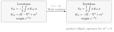
After integration by parts, $S_M=-\frac12\int\phi(\partial_t^2-\nabla^2+m^2)\phi$. Wick rotation converts this Lorentzian equation-of-motion operator, together with the contour measure, into the positive Euclidean quadratic form $S_E=\frac12\int\phi(-\partial_\tau^2-\nabla^2+m^2)\phi$. The weight changes from $e^{iS_M}$ to the damped Gaussian $e^{-S_E}$.

The free Euclidean propagator

The free Euclidean scalar action is

$$S_{E,0}[\phi] =\frac12\int d^4x_E\,\phi(x) \left(-\partial_E^2+m^2\right) \phi(x),$$

where

$$\partial_E^2=\partial_\tau^2+\nabla^2, \qquad x_E=(\tau,\mathbf x).$$

The Euclidean propagator is the inverse of the positive operator

$$K_E=-\partial_E^2+m^2.$$

Thus

$$K_EG_E(x-y)=\delta^{(4)}(x-y),$$

and in momentum space

$$\boxed{ \widetilde G_E(p_E)={1\over p_E^2+m^2}, \qquad p_E^2=p_4^2+\mathbf p^2. }$$

This is the Euclidean version of the Feynman propagator. The safest practical dictionary is not just a denominator replacement, but a contour-and-measure replacement:

$$\int {dp^0\over2\pi}\,{i\over (p^0)^2-E_{\mathbf p}^2+i0} \quad\longrightarrow\quad \int {dp_4\over2\pi}\,{1\over p_4^2+E_{\mathbf p}^2}.$$

The Lorentzian denominator $p^2-m^2+i0$ becomes $-(p_E^2+m^2)$ after the contour rotation, while $dp^0=i\,dp_4$ and the numerator $i$ combine to leave a positive Euclidean Gaussian inverse. In practice, Euclidean perturbation theory therefore uses

$${1\over p_E^2+m^2}$$

as the scalar line.

Do not Wick rotate on-shell kinematics blindly

For internal loop energies, Wick rotation is a contour deformation controlled by the $i0$ prescription. For external scattering momenta, one usually computes an analytic Euclidean function and only later continues the appropriate invariants back to physical Minkowski values. Replacing every real on-shell energy by $ip_4$ inside a scattering formula is not a valid shortcut.

A useful check is the mixed representation, provided the analytic branches are kept explicit. For $t>0$ the Lorentzian time-ordered propagator contains $e^{-iE_{\mathbf p}t}/(2E_{\mathbf p})$ and is continued through the lower imaginary-time quadrant. For $t<0$ its oppositely ordered branch is continued separately. Reassembling the two Euclidean branches gives

$$G_E(\tau,\mathbf p) =\frac{e^{-E_{\mathbf p}|\tau|}}{2E_{\mathbf p}}.$$

One should not treat $|t|$ itself as a holomorphic function and substitute $t=-i\tau$ into it.

A one-dimensional version is especially transparent. For the Euclidean harmonic oscillator

$$S_E[q]=\int d\tau\,\frac12\left[\dot q(\tau)^2+\Omega^2q(\tau)^2\right],$$

the Green function obeys

$$\left(-{d^2\over d\tau^2}+\Omega^2\right)G_E(\tau)=\delta(\tau).$$

Fourier transforming gives

$$G_E(\tau) =\int_{-\infty}^{\infty}{d\omega\over2\pi}\,{e^{i\omega\tau}\over \omega^2+\Omega^2} ={1\over2\Omega}e^{-\Omega|\tau|}.$$

The exponential decay is the Euclidean imprint of the oscillator energy gap.

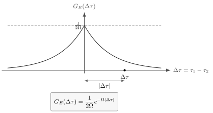
The Euclidean oscillator propagator $G_E(\tau)=e^{-\Omega|\tau|}/(2\Omega)$ is the inverse of $-\partial_\tau^2+\Omega^2$. Unlike the Lorentzian propagator, it decays at large separation instead of oscillating.

Gaussian generating functional

Introduce a Euclidean source $J(x)$ by

$$Z_E[J]=\int\mathcal D\phi\, \exp\left[-S_{E,0}[\phi]+\int d^4x_E\,J(x)\phi(x)\right].$$

First keep finite ultraviolet and volume regulators, so the independent real field variables form a vector $q\in\mathbb R^n$. Assume the regulated quadratic matrix $K$ is real symmetric and positive definite. A massive free scalar with compatible boundary conditions has this property; a massless constant mode must be fixed, removed, or regulated before using $K^{-1}$. For real source $J$, the Gaussian identity with ordinary Lebesgue measure is

$$\int d^nq\,\exp\left[-\frac12q_iK_{ij}q_j+J_iq_i\right] =(2\pi)^{n/2}(\det K)^{-1/2} \exp\left[\frac12J_iK^{-1}_{ij}J_j\right].$$

Completing the square with $q\mapsto q+K^{-1}J$ gives the source exponent; orthogonally diagonalizing $K$ gives the determinant and the factor $(2\pi)^{n/2}$. The regulated Gaussian treatment develops this finite-dimensional starting point. Dividing by the zero-source integral cancels its normalization and gives the functional notation

$$\boxed{ {Z_E[J]\over Z_E[0]} =\exp\left[\frac12\int d^4x_E\,d^4y_E\, J(x)G_E(x-y)J(y)\right]. }$$

Correlation functions follow by differentiating with respect to $J$:

$$\langle\phi(x_1)\cdots\phi(x_n)\rangle_E =\left.{1\over Z_E[0]}{\delta^nZ_E[J]\over\delta J(x_1)\cdots\delta J(x_n)}\right|_{J=0}.$$

Notice the absence of extra powers of $i$. In Lorentzian signature the normalized source functional uses $e^{iS+i\int J\phi}$, while the Euclidean functional uses $e^{-S_E+\int J\phi}$. This is a small difference, but it prevents many sign mistakes when translating Schwinger–Dyson identities and Feynman rules.

For the free theory, this immediately reproduces Wick’s theorem. The two-point function is $G_E(x-y)$, odd-point functions vanish, and the four-point function is

$$\begin{aligned} \langle\phi_1\phi_2\phi_3\phi_4\rangle_E &=G_{12}G_{34}+G_{13}G_{24}+G_{14}G_{23}, \end{aligned}$$

where $G_{ij}=G_E(x_i-x_j)$.

The Gaussian determinant $Z_E[0]\propto(\det K_E)^{-1/2}$ contains the vacuum functional. In perturbative calculations normalized correlators often divide by $Z_E[0]$, so this determinant cancels. When computing vacuum energies, effective actions, or finite-temperature free energies, it becomes physically important.

Euclidean Schwinger–Dyson identities

Euclidean path integrals also make the equation-of-motion identities very clean. Let $F[\phi]$ be a product of fields. Assuming that functional integration by parts has no boundary term,

$$0=\int\mathcal D\phi\,{\delta\over\delta\phi(x)} \left(e^{-S_E[\phi]}F[\phi]\right).$$

Expanding the derivative gives

$$\boxed{ \left\langle {\delta S_E\over\delta\phi(x)}F[\phi]\right\rangle_E =\left\langle {\delta F[\phi]\over\delta\phi(x)}\right\rangle_E. }$$

For the free scalar theory,

$${\delta S_{E,0}\over\delta\phi(x)}=(-\partial_E^2+m^2)\phi(x).$$

Choosing

$$F[\phi]=\phi(x_2)\cdots\phi(x_n)$$

gives

$$(-\partial_{x_1,E}^2+m^2) \langle\phi(x_1)\phi(x_2)\cdots\phi(x_n)\rangle_E =\sum_{j=2}^{n}\delta^{(4)}(x_1-x_j) \langle\phi(x_2)\cdots\widehat{\phi(x_j)}\cdots\phi(x_n)\rangle_E.$$

The hat means that the field is omitted. For $n=2$ this is just the Green-function equation

$$(-\partial_E^2+m^2)G_E(x-y)=\delta^{(4)}(x-y).$$

For $n=4$ it gives the recursion behind Wick’s theorem: acting with the inverse propagator on one external point collapses that point onto each of the others.

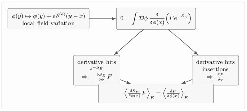
The Euclidean Schwinger–Dyson identity is functional integration by parts. In a free theory, $K_E$ acting on one leg of an $n$-point function produces contact terms where that point coincides with one of the other insertions.

This equation is the Euclidean counterpart of the contact-term identities that appeared in Lorentzian time-ordered products. The difference is that no time-ordering step functions are needed in the Euclidean path-integral derivation; the contact terms come directly from differentiating the inserted fields.

Spectral decay and mass extraction

Euclidean correlation functions remember the energy spectrum. For a Hermitian operator $\mathcal O$ with the quantum numbers of some particle, first remove a possible vacuum expectation value,

$$\widehat{\mathcal O}=\mathcal O-\langle\mathcal O\rangle_E.$$

Then consider the connected zero-momentum two-point function

$$C(\tau)=\int d^3x\,\langle \widehat{\mathcal O}(\tau,\mathbf x)\widehat{\mathcal O}(0,\mathbf 0)\rangle_E, \qquad \tau>0.$$

Insert a complete set of Hamiltonian eigenstates:

$$C(\tau)=\sum_{n\ne0} A_n e^{-(E_n-E_0)\tau},$$

where $A_n\ge0$ includes the state-normalization and zero-momentum-projection factors. With the covariant one-particle normalization used on the preceding pages, an isolated state contributes $A_n=|\langle0|\widehat{\mathcal O}(0)|n,\mathbf0\rangle|^2/(2E_{n,\mathbf0})$. In finite volume the same statement is a literal discrete sum with unit-normalized states.

At large $\tau$, the lowest state with nonzero overlap dominates:

$$C(\tau)\sim A e^{-M\tau}.$$

Thus masses appear as exponential decay rates in Euclidean time. This fact is the operational heart of Euclidean lattice field theory: one computes Euclidean correlators and reads off spectra from their long-distance decay. In infinite volume a multiparticle sector becomes a continuum and contributes a spectral integral rather than a discrete sum; an isolated stable state still produces the single exponential displayed above.

For a free scalar field at spatial momentum $\mathbf p$,

$$G_E(\tau,\mathbf p) ={1\over2E_{\mathbf p}}e^{-E_{\mathbf p}|\tau|}, \qquad E_{\mathbf p}=\sqrt{\mathbf p^2+m^2}.$$

This is the same formula as the harmonic oscillator result with $\Omega=E_{\mathbf p}$. A free field is again an infinite collection of oscillators, one for each momentum mode.

The statistical-mechanics viewpoint

A classical statistical system with Hamiltonian $H(p,q)$ has partition function

$$Z_{\mathrm{cl}}=\int \prod_i dp_i\,dq_i\,e^{-\beta H(p,q)}.$$

If

$$H(p,q)=\sum_i {p_i^2\over2m}+V(q),$$

then the momenta are Gaussian and can be integrated out:

$$Z_{\mathrm{cl}}\propto\int\prod_i dq_i\,e^{-\beta V(q)}.$$

The Euclidean QFT expression

$$Z_E=\int\mathcal D\phi\,e^{-S_E[\phi]}$$

has precisely this form, with the field configuration $\phi(x_E)$ playing the role of a statistical configuration and $S_E$ playing the role of an energy functional. This analogy is not just poetic. It is the reason the same mathematics describes scalar QFT, magnets near criticality, Euclidean random fields, and lattice models.

For example, the Euclidean scalar action

$$S_E[\phi]=\int d^dx\left[\frac12(\nabla\phi)^2+\frac12r\phi^2+\frac{u}{4!}\phi^4\right]$$

is also the Landau–Ginzburg free-energy functional for an order parameter. In relativistic QFT one often thinks of $d$ as Euclidean spacetime dimension; in statistical mechanics one often thinks of $d$ as ordinary spatial dimension. The mathematics of the functional integral is the same.

The next pages develop this idea more explicitly: first by comparing field theory with statistical mechanics, then by studying critical behavior, thermal masses, and the compact imaginary-time circle.

Summary

Wick rotation turns real time into imaginary time, $t=-i\tau$. With the Feynman prescription, positive-energy factors $e^{-iEt}$ become damped factors $e^{-E\tau}$. This turns the Lorentzian weight $e^{iS}$ into the Euclidean weight $e^{-S_E}$.

For a scalar field, the Euclidean action is positive in the free massive theory:

$$S_{E,0}=\frac12\int d^4x_E\,\phi(-\partial_E^2+m^2)\phi.$$

The free Euclidean propagator is the inverse operator

$$\widetilde G_E(p_E)={1\over p_E^2+m^2},$$

and the Gaussian generating functional is

$${Z_E[J]\over Z_E[0]} =\exp\left[\frac12\int JG_EJ\right].$$

Euclidean correlation functions decay exponentially at large time separation. Their decay rates are energy gaps, so particle masses become measurable from long-distance Euclidean behavior. The same formalism also exposes the deep relation between QFT and statistical mechanics: $S_E$ plays the role of a Boltzmann energy functional.

Common pitfalls

A Wick rotation is not merely replacing $t$ by $\tau$ in a formula. The direction of the contour and the $i0$ prescription decide which exponential is damped and which would blow up.

Do not mix Lorentzian and Euclidean propagators in the same expression. In the conventions of this course,

$$\widetilde G_F(p)={i\over p^2-m^2+i0}, \qquad \widetilde G_E(p_E)={1\over p_E^2+m^2}.$$

They are related by analytic continuation, but they are not the same function written in different notation.

Euclidean time is not an extra physical time. It is a calculational and structural continuation. Real-time causal questions require analytic continuation back to Lorentzian signature.

Do not rotate only the denominator while forgetting the integration contour and measure. The familiar Euclidean line $1/(p_E^2+m^2)$ comes from the full contour rotation of the Feynman integral, not from an isolated algebraic substitution.

Finally, not every Euclidean functional integral defines a healthy Lorentzian quantum theory. Reflection positivity, locality, and appropriate analyticity conditions are needed to reconstruct a unitary Lorentzian theory.

Exercises

Exercise 1

Starting from

$$S=\int dt\,\left[\frac12\dot q^2-\frac12\Omega^2q^2-{\lambda\over4!}q^4\right],$$

perform the Wick rotation $t=-i\tau$ and derive the Euclidean action.

Solution

Under $t=-i\tau$,

$$dt=-i\,d\tau, \qquad \dot q={dq\over dt}=i{dq\over d\tau}=iq'.$$

Therefore

$$\dot q^2=-(q')^2.$$

The Lorentzian action becomes

$$S=-i\int d\tau\left[-\frac12(q')^2-\frac12\Omega^2q^2-{\lambda\over4!}q^4\right] =i\int d\tau\left[\frac12(q')^2+\frac12\Omega^2q^2+{\lambda\over4!}q^4\right].$$

Thus $S=iS_E$, where

$$S_E=\int d\tau\left[\frac12(q')^2+\frac12\Omega^2q^2+{\lambda\over4!}q^4\right].$$

Hence $e^{iS}=e^{-S_E}$.

Exercise 2

Show that

$$G_E(\tau)=\int_{-\infty}^{\infty}{d\omega\over2\pi}\,{e^{i\omega\tau}\over\omega^2+\Omega^2}$$

equals $e^{-\Omega|\tau|}/(2\Omega)$.

Solution

For $\tau>0$, close the contour in the upper half-plane because $e^{i\omega\tau}$ decays there. The pole is at $\omega=i\Omega$, and its residue is

$$\operatorname{Res}_{\omega=i\Omega}{e^{i\omega\tau}\over\omega^2+\Omega^2} ={e^{-\Omega\tau}\over2i\Omega}.$$

The integral is

$$G_E(\tau)=i\,{e^{-\Omega\tau}\over2i\Omega}={1\over2\Omega}e^{-\Omega\tau}.$$

For $\tau<0$, close the contour in the lower half-plane. The pole is at $\omega=-i\Omega$, and the clockwise orientation gives the same final form with $\tau$ replaced by $|\tau|$:

$$G_E(\tau)={1\over2\Omega}e^{-\Omega|\tau|}.$$

Exercise 3

Use the Euclidean Schwinger–Dyson identity to show that the harmonic-oscillator two-point function obeys

$$\left(-{d^2\over d\tau^2}+\Omega^2\right)\langle q(\tau)q(\tau')\rangle_E=\delta(\tau-\tau').$$

Solution

For

$$S_E[q]=\int d\tau\,{1\over2}\left(\dot q^2+\Omega^2q^2\right),$$

integration by parts gives

$${\delta S_E\over\delta q(\tau)}=\left(-{d^2\over d\tau^2}+\Omega^2\right)q(\tau).$$

Use

$$0=\int\mathcal Dq\,{\delta\over\delta q(\tau)}\left(e^{-S_E[q]}q(\tau')\right).$$

Expanding the derivative,

$$0=-\left\langle {\delta S_E\over\delta q(\tau)}q(\tau')\right\rangle_E+\left\langle {\delta q(\tau')\over\delta q(\tau)}\right\rangle_E.$$

Since

$${\delta q(\tau')\over\delta q(\tau)}=\delta(\tau-\tau'),$$

we obtain

$$\left(-{d^2\over d\tau^2}+\Omega^2\right)\langle q(\tau)q(\tau')\rangle_E=\delta(\tau-\tau').$$

Exercise 4

Let

$$C(\tau)=\sum_n A_n e^{-E_n\tau}, \qquad 0<E_0<E_1<\cdots, \qquad A_0\neq0.$$

Show that the effective mass

$$M_{\mathrm{eff}}(\tau)=-{d\over d\tau}\log C(\tau)$$

approaches $E_0$ as $\tau\to\infty$.

Solution

Factor out the lowest exponential:

$$C(\tau)=A_0e^{-E_0\tau}\left[1+\sum_{n\ge1}{A_n\over A_0}e^{-(E_n-E_0)\tau}\right].$$

Taking the logarithm,

$$\log C(\tau)=\log A_0-E_0\tau+ \log\left[1+\sum_{n\ge1}{A_n\over A_0}e^{-(E_n-E_0)\tau}\right].$$

The final logarithm approaches zero exponentially fast because every $E_n-E_0$ is positive. Therefore

$$M_{\mathrm{eff}}(\tau)=-{d\over d\tau}\log C(\tau) \to E_0.$$

This is the basic mass-extraction idea used in Euclidean correlator methods.

Further reading

• Sidney Coleman, Lectures on Quantum Field Theory, edited by Bryan Gin-ge Chen et al., World Scientific, 2019, chapter 28.
• Mark Srednicki, Quantum Field Theory, Cambridge University Press, 2007, chapters 8–9.
• Steven Weinberg, The Quantum Theory of Fields, Volume I: Foundations, Cambridge University Press, 1995, chapter 9.
• A. Zee, Quantum Field Theory in a Nutshell, 2nd edition, Princeton University Press, 2010, chapters I.2 and V.2.