Imaginary Time and Matsubara Propagators

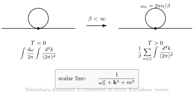
The Euclidean path integral was introduced in the previous pages as a way to turn oscillatory amplitudes into convergent weights. This page adds one more ingredient: temperature. The partition function of a quantum system is a trace,

$$Z(\beta)=\operatorname{Tr}\,e^{-\beta H}, \qquad \beta={1\over T},$$

and a trace is what turns Euclidean time into a circle. The basic replacement is not merely formal. Real-time evolution contains $e^{-iHt}$; thermal weighting contains $e^{-\beta H}$. Thus thermal field theory is obtained by evolving through imaginary time of length $\beta$ and identifying the final state with the initial state.

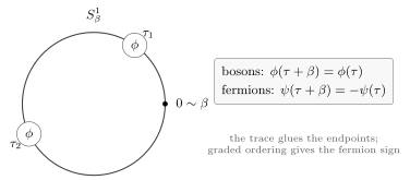
For bosonic fields this identification is periodic,

$$\phi(\tau+\beta,\mathbf x)=\phi(\tau,\mathbf x),$$

whereas for fermionic fields it is antiperiodic. This single boundary condition is responsible for Matsubara frequencies, thermal propagators, Bose and Fermi occupation numbers, and the finite-temperature Feynman rules.

A useful early dictionary is:

object	direct meaning
$G^>(t)=\langle\phi(t)\phi(0)\rangle_\beta$	real-time fluctuation with one operator later than the other
$G^<(t)=\langle\phi(0)\phi(t)\rangle_\beta$	the reversed Wightman ordering
$G_E(\tau)=\langle T_\tau\phi(\tau)\phi(0)\rangle_\beta$	the imaginary-time correlator computed by Matsubara sums
$G_R(t)=i\theta(t)\langle[\phi(t),\phi(0)]\rangle_\beta$	the causal response convention used in this course

The imaginary-time formalism computes $G_E$ directly. Real-time response requires the KMS relation plus analytic continuation.

Thermal traces and imaginary-time evolution

Thermal circle and Matsubara normalization

The page uses Euclidean time $t=-i\tau$ in thermal formulas, with $0\le \tau<\beta$. Here $d$ denotes the number of spatial dimensions, so the Euclidean thermal spacetime is $S^1_\beta\times\mathbb R^d$. Spatial momentum integrals are abbreviated as

$$\int_{\mathbf k} f(\mathbf k) =\int {d^d k\over (2\pi)^d}\,f(\mathbf k),$$

and bosonic Matsubara frequencies are

$$\omega_n={2\pi n\over \beta}=2\pi nT, \qquad n\in\mathbb Z.$$

For a free scalar mode,

$$E_{\mathbf k}=\sqrt{\mathbf k^2+m^2}.$$

A thermal expectation value is

$$\langle \mathcal O\rangle_\beta ={1\over Z}\operatorname{Tr}\left(e^{-\beta H}\mathcal O\right), \qquad Z=\operatorname{Tr}\,e^{-\beta H}.$$

The trace is cyclic:

$$\operatorname{Tr}(ABC)=\operatorname{Tr}(BCA)=\operatorname{Tr}(CAB),$$

provided the products are well-defined. This innocent-looking identity is the algebraic origin of thermal periodicity. In the Heisenberg picture,

$$A(t)=e^{iHt}A(0)e^{-iHt}.$$

Analytically continuing to imaginary time gives

$$A(\tau)=e^{\tau H}A(0)e^{-\tau H}.$$

The thermal trace then lets an operator move around the circle:

$$\operatorname{Tr}\left(e^{-\beta H}A(\tau)B(0)\right) =\operatorname{Tr}\left(e^{-\beta H}B(0)A(\tau-\beta)\right).$$

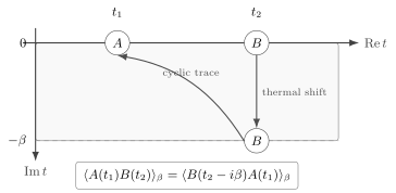
Equivalently, for real time one obtains the Kubo–Martin–Schwinger condition,

$$\boxed{ G^>(t-i\beta)=G^<(t), }$$

where

$$G^>(t)=\langle A(t)B(0)\rangle_\beta, \qquad G^<(t)=\langle B(0)A(t)\rangle_\beta.$$

For bosonic operators at Euclidean time this becomes periodicity of the imaginary-time ordered two-point function. There is an important subtlety for fermions: the ordinary Hilbert-space trace is still cyclic and does not acquire a graded sign. The minus sign instead comes from graded imaginary-time ordering (equivalently, from the fermionic coherent-state representation of the trace). For $0<\tau<\beta$, cyclicity gives

$$\langle\psi(\tau)\bar\psi(0)\rangle_\beta =\langle\bar\psi(0)\psi(\tau-\beta)\rangle_\beta,$$

but $T_\tau$ contributes a minus sign on the right because $\tau-\beta<0$. Hence $S_E(\tau)\equiv\langle T_\tau\psi(\tau)\bar\psi(0)\rangle_\beta$ satisfies $S_E(\tau-\beta)=-S_E(\tau)$.

The trace $\operatorname{Tr}\,e^{-\beta H}$ identifies the end of the Euclidean-time interval with its beginning. Bosonic fields live on a circle of circumference $\beta$, while fermionic fields pick up a minus sign after one winding.

The path-integral version follows from inserting complete sets of field eigenstates between short Euclidean time steps. For bosons,

$$\boxed{ Z(\beta)=\operatorname{Tr}\,e^{-\beta H} =\int_{\phi(\beta)=\phi(0)}\mathcal D\phi\,e^{-S_E[\phi]}. }$$

For a scalar field,

$$S_E[\phi] =\int_0^\beta d\tau\int d^d x\, \left[ {1\over2}(\partial_\tau\phi)^2 +{1\over2}(\nabla\phi)^2 +{1\over2}m^2\phi^2 +V_{\mathrm{int}}(\phi) \right].$$

The zero-temperature Euclidean theory is recovered by sending $\beta\to\infty$. Then the thermal circle opens into the full Euclidean time line.

KMS condition and detailed balance

The same trace identity is also the field-theoretic version of detailed balance. Suppose a system is weakly coupled to a probe through an interaction of the schematic form

$$H_{\mathrm{int}}(t)=-M(t)\,\phi(t,\mathbf 0),$$

where $M(t)$ is an external source or detector variable. The transition rate contains the Fourier transform of a thermal Wightman function. Define

$$G^>(t)=\langle \phi(t)\phi(0)\rangle_\beta, \qquad G^<(t)=\langle \phi(0)\phi(t)\rangle_\beta.$$

Insert a complete set of exact energy eigenstates:

$$G^>(t) ={1\over Z}\sum_{m,n}e^{-\beta E_n} |\langle m|\phi|n\rangle|^2 e^{-i(E_m-E_n)t}.$$

Using the Fourier convention

$$G^>(\omega)=\int_{-\infty}^\infty dt\,e^{i\omega t}G^>(t),$$

we obtain

$$G^>(\omega) ={2\pi\over Z}\sum_{m,n}e^{-\beta E_n} |\langle m|\phi|n\rangle|^2 \delta(\omega-E_m+E_n).$$

Similarly,

$$G^<(\omega) ={2\pi\over Z}\sum_{m,n}e^{-\beta E_m} |\langle m|\phi|n\rangle|^2 \delta(\omega-E_m+E_n).$$

On the support of the delta function, $E_m-E_n=\omega$, so

$$e^{-\beta E_m}=e^{-\beta \omega}e^{-\beta E_n}.$$

Therefore

$$\boxed{ G^<(\omega)=e^{-\beta\omega}G^>(\omega). }$$

Equivalently,

$$G^>(\omega)=e^{\beta\omega}G^<(\omega).$$

This is the frequency-space form of the KMS condition.

Thermal correlators are naturally analytic in a strip of complex time. Moving an operator by $-i\beta$ around the strip is equivalent, by cyclicity of the trace, to exchanging its order inside the thermal average: $G^>(t-i\beta)=G^<(t)$.

The spectral function is

$$\rho(\omega,\mathbf k) =G^>(\omega,\mathbf k)-G^<(\omega,\mathbf k).$$

For $\omega>0$, the KMS relation gives

$$G^>(\omega,\mathbf k) =\left(1+n_B(\omega)\right)\rho(\omega,\mathbf k), \qquad G^<(\omega,\mathbf k) =n_B(\omega)\rho(\omega,\mathbf k),$$

where

$$\boxed{ n_B(\omega)={1\over e^{\beta\omega}-1}. }$$

The factor $1+n_B$ is the Bose enhancement factor. The $1$ is spontaneous emission; the $n_B$ is stimulated emission by quanta already present in the thermal bath. Absorption is proportional to $n_B$. In equilibrium these two processes obey detailed balance.

For a transition $A\to B$ with energy absorbed by the system

$$\omega=E_B-E_A,$$

detailed balance says

$$\boxed{ {W_{A\to B}\over W_{B\to A}}=e^{-\beta\omega}. }$$

Upward transitions are Boltzmann suppressed. Downward transitions are favored, but in equilibrium the larger occupation probability of the lower state compensates exactly.

Imaginary-time ordered Green functions

Thermal perturbation theory uses Euclidean time-ordering. For bosonic operators,

$$T_\tau A(\tau_1)B(\tau_2) = \begin{cases} A(\tau_1)B(\tau_2),&\tau_1>\tau_2,\\ B(\tau_2)A(\tau_1),&\tau_2>\tau_1. \end{cases}$$

The thermal Euclidean two-point function is

$$G_E(\tau_1,\tau_2) =\langle T_\tau\phi(\tau_1)\phi(\tau_2)\rangle_\beta.$$

Thermal equilibrium is time-translation invariant, so $G_E$ depends only on

$$\tau=\tau_1-\tau_2$$

modulo $\beta$. Bosonic periodicity gives

$$G_E(\tau+\beta)=G_E(\tau).$$

For a single harmonic oscillator of frequency $m$, or for one scalar momentum mode with $m$ replaced by $E_{\mathbf k}$, the operator is

$$q(\tau)={1\over\sqrt{2m}} \left(ae^{-m\tau}+a^\dagger e^{m\tau}\right),$$

and the thermal averages are

$$\langle a^\dagger a\rangle_\beta=n_B(m), \qquad \langle aa^\dagger\rangle_\beta=1+n_B(m).$$

For $0<\tau<\beta$,

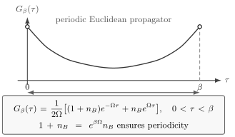
$$\boxed{ G_E(\tau) ={1\over 2m} \left[(1+n_B(m))e^{-m\tau}+n_B(m)e^{m\tau}\right]. }$$

Since

$$n_B(m)={1\over e^{\beta m}-1},$$

this may also be written as

$$\boxed{ G_E(\tau) ={1\over 2m} {\cosh\left[m\left({\beta\over2}-\tau\right)\right] \over \sinh(\beta m/2)}, \qquad 0\le \tau\le \beta. }$$

Here $\tau$ is the representative of the separation on the thermal circle chosen in the interval $0\le\tau\le\beta$. The correlator satisfies

$$\left(-\partial_\tau^2+m^2\right)G_E(\tau) =\delta_\beta(\tau),$$

where $\delta_\beta$ is the periodic delta function on the circle,

$$\delta_\beta(\tau)=\sum_{\ell\in\mathbb Z}\delta(\tau-\ell\beta).$$

The finite-temperature propagator can be viewed as the zero-temperature Euclidean propagator plus images winding around the thermal circle. For a harmonic oscillator, this gives $G_E(\tau)=(2m)^{-1}[(1+n_B)e^{-m\tau}+n_Be^{m\tau}]$ for $0<\tau<\beta$.

At zero temperature, $\beta\to\infty$ and $n_B(m)\to0$. The propagator reduces to the vacuum Euclidean propagator

$$G_E(\tau)\longrightarrow {1\over 2m}e^{-m|\tau|}.$$

At high temperature, $\beta m\ll1$, the occupation number becomes

$$n_B(m)\simeq {T\over m},$$

so thermal fluctuations dominate over the zero-point contribution.

Matsubara frequencies

A function on a circle has a Fourier series, not a continuous Fourier transform. Bosonic periodicity requires

$$e^{i\omega_n\beta}=1,$$

so

$$\boxed{ \omega_n={2\pi n\over\beta}=2\pi nT, \qquad n\in\mathbb Z. }$$

These are the bosonic Matsubara frequencies. Fermionic antiperiodicity requires $e^{i\omega_n\beta}=-1$, so fermions have

$$\omega_n^{(F)}={(2n+1)\pi\over\beta}=(2n+1)\pi T.$$

For a free scalar field,

$$\phi(\tau,\mathbf x) ={1\over\sqrt\beta} \sum_{n\in\mathbb Z} \int_{\mathbf k} e^{i\mathbf k\cdot\mathbf x-i\omega_n\tau} \phi_n(\mathbf k).$$

The Euclidean quadratic action becomes diagonal:

$$S_{E,0} ={1\over2}\sum_{n\in\mathbb Z}\int_{\mathbf k} \left(\omega_n^2+\mathbf k^2+m^2\right) \phi_n(\mathbf k)\phi_{-n}(-\mathbf k).$$

Thus the free Matsubara propagator is

$$\boxed{ G_E(\omega_n,\mathbf k) ={1\over \omega_n^2+E_{\mathbf k}^2}, \qquad E_{\mathbf k}^2=\mathbf k^2+m^2. }$$

In mixed representation,

$$\boxed{ G_E(\tau,\mathbf k) ={1\over\beta}\sum_{n\in\mathbb Z} {e^{-i\omega_n\tau}\over \omega_n^2+E_{\mathbf k}^2}. }$$

Evaluating the sum gives exactly the thermal oscillator formula with $m\to E_{\mathbf k}$:

$$G_E(\tau,\mathbf k) ={1\over2E_{\mathbf k}} \left[(1+n_B(E_{\mathbf k}))e^{-E_{\mathbf k}\tau} +n_B(E_{\mathbf k})e^{E_{\mathbf k}\tau} \right], \qquad 0<\tau<\beta.$$

Compact Euclidean time discretizes energy. Bosons have $\omega_n=2\pi nT$ and include a zero mode. Fermions have $\omega_n=(2n+1)\pi T$ and therefore no zero mode.

The delta function on the circle is also a Fourier series:

$$\delta_\beta(\tau) ={1\over\beta}\sum_{n\in\mathbb Z}e^{-i\omega_n\tau}.$$

Applying $-\partial_\tau^2+E_{\mathbf k}^2$ to the Matsubara representation gives

$$\left(-\partial_\tau^2+E_{\mathbf k}^2\right)G_E(\tau,\mathbf k) ={1\over\beta}\sum_n e^{-i\omega_n\tau} =\delta_\beta(\tau),$$

which is the Green-function equation on the thermal circle.

Finite-temperature Feynman rules

The imaginary-time formalism gives perturbation theory that looks almost identical to Euclidean zero-temperature perturbation theory. The changes are precise:

1. Euclidean time is compact: $0\le \tau<\beta$.
2. Bosonic fields are periodic and fermionic fields are antiperiodic.
3. Energy integrals are replaced by Matsubara sums.

With the integral convention of this page,

$$\boxed{ \int {dk_0\over2\pi}\int_{\mathbf k} \quad\longrightarrow\quad T\sum_{n\in\mathbb Z}\int_{\mathbf k} }$$

for a bosonic loop. The scalar propagator becomes

$${1\over k_0^2+\mathbf k^2+m^2} \quad\longrightarrow\quad {1\over \omega_n^2+\mathbf k^2+m^2}.$$

At finite temperature, Euclidean energy is discrete. In loop diagrams the continuous integral over $k_0$ is replaced by a Matsubara sum, while spatial momentum remains continuous in infinite volume.

For example, the one-loop tadpole that shifted the mass in the previous page becomes, at finite temperature,

$$\Pi_\beta ={\lambda\over2} T\sum_{n\in\mathbb Z} \int_{\mathbf k} {1\over \omega_n^2+E_{\mathbf k}^2}.$$

The Matsubara sum identity

$$T\sum_{n\in\mathbb Z}{1\over \omega_n^2+E^2} ={1\over2E}\left(1+2n_B(E)\right)$$

splits this loop into a zero-temperature part and a genuine thermal part:

$$\Pi_\beta ={\lambda\over2}\int_{\mathbf k}{1\over2E_{\mathbf k}} +{\lambda\over2}\int_{\mathbf k}{n_B(E_{\mathbf k})\over E_{\mathbf k}}.$$

The first term is the familiar vacuum fluctuation. The second term is the thermal population of real modes in the heat bath.

In a massless scalar theory in three spatial dimensions,

$$\int_{\mathbf k}{n_B(|\mathbf k|)\over |\mathbf k|} ={T^2\over12},$$

so the leading thermal mass correction is

$$\Delta m_T^2={\lambda T^2\over24}$$

for the interaction $\lambda\phi^4/4!$. The numerical coefficient depends on the normalization of the quartic interaction, but the scaling $\Delta m_T^2\sim \lambda T^2$ is robust.

Dimensional reduction at high temperature

Matsubara frequencies reveal a useful physical picture. At high temperature, the gap between nonzero Matsubara frequencies is

$$2\pi T.$$

For static, long-distance phenomena with characteristic momenta $k\ll 2\pi T$, all modes with $n\ne0$ are heavy. The bosonic zero mode $\omega_0=0$ dominates infrared physics. A $(d+1)$-dimensional Euclidean finite-temperature theory then reduces, at sufficiently long distances, to an effective $d$-dimensional statistical field theory for the zero mode:

$$\phi(\tau,\mathbf x) \approx \phi_0(\mathbf x).$$

This is the field-theoretic meaning of the slogan:

$$\text{high-temperature quantum field theory} \quad\longrightarrow\quad \text{classical statistical field theory in one fewer dimension}.$$

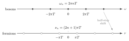
Fermions do not have zero modes because their Matsubara frequencies are odd multiples of $\pi T$. This is one reason finite-temperature bosonic infrared physics is often more singular than fermionic infrared physics.

The zero mode should not be confused with the vacuum mode. It is a Fourier mode around the thermal circle, not a state in the Hilbert space. Its importance is kinematic: it is the only mode whose Matsubara frequency does not itself provide an effective mass.

Analytic continuation back to real time

Matsubara correlators are Euclidean objects. They compute equilibrium thermodynamics and imaginary-time correlation functions. Real-time response functions are obtained by analytic continuation, but this is a convention-sensitive step.

For the free scalar convention used in this course,

$$G_E(\omega_n,\mathbf k)={1\over\omega_n^2+E_{\mathbf k}^2}.$$

Earlier we used the retarded response convention

$$G_R(t)=i\theta(t)\langle[\phi(t),\phi(0)]\rangle_\beta,$$

which gives a positive delta-function source in the equation of motion. With the Fourier convention $G_R(t)=\int d\omega\,e^{-i\omega t}G_R(\omega)/(2\pi)$, the free retarded propagator is therefore

$$G_R(\omega,\mathbf k) ={1\over E_{\mathbf k}^2-(\omega+i0)^2}.$$

Thus the direct free-field continuation is

$$\boxed{ G_R(\omega,\mathbf k) =G_E\left(\omega_n\to -i(\omega+i0),\mathbf k\right). }$$

Many books define the retarded function with the opposite overall sign, $G_R^{\mathrm{alt}}(t)=-i\theta(t)[\phi(t),\phi(0)]$. In that convention the same pole prescription appears with an overall minus sign. The pole location $\omega\to\omega+i0$ is the invariant content; the overall sign follows the definition of the real-time response function.

A cleaner way to state the analytic structure is to keep the definitions on this page fixed. We defined

$$\rho(\omega,\mathbf k) =\int_{-\infty}^{\infty}dt\,e^{i\omega t} \langle[\phi(t,\mathbf k),\phi(0,-\mathbf k)]\rangle_\beta$$

and use the nonstandard-but-consistent response convention $G_R=+i\theta\langle[\phi,\phi]\rangle_\beta$. Introduce the analytic function

$$\mathcal G(z,\mathbf k) =\int_{-\infty}^{\infty}{d\omega'\over2\pi} {\rho(\omega',\mathbf k)\over z-\omega'}.$$

The definitions then fix both signs:

$$\boxed{ G_R(\omega,\mathbf k)=-\mathcal G(\omega+i0,\mathbf k), \qquad G_E(\omega_n,\mathbf k)=-\mathcal G(i\omega_n,\mathbf k). }$$

For example, the free scalar spectral density is

$$\rho_0(\omega,\mathbf k) ={\pi\over E_{\mathbf k}} \left[\delta(\omega-E_{\mathbf k})-\delta(\omega+E_{\mathbf k})\right],$$

so $\mathcal G_0(z,\mathbf k)=1/(z^2-E_{\mathbf k}^2)$. The two boxed relations reproduce both $G_E=1/(\omega_n^2+E_{\mathbf k}^2)$ and $G_R=1/[E_{\mathbf k}^2-(\omega+i0)^2]$. This is why many references write the slogan $i\omega_n\to\omega+i0$: it applies naturally to the analytic variable $z$, while the direct continuation of the real Matsubara label in our displayed Euclidean formula is $\omega_n\to-i(\omega+i0)$. Definitions must be checked before comparing overall signs.

Euclidean correlators are known only at discrete Matsubara frequencies, so reconstructing the full spectral density from Euclidean data is an analytic continuation problem, not an algebraic substitution. In perturbation theory, however, one often computes an analytic expression in the complex frequency variable and then takes the appropriate retarded boundary value.

Summary

Finite temperature turns Euclidean time into a compact direction. The trace $\operatorname{Tr}\,e^{-\beta H}$ imposes periodic boundary conditions on bosons and antiperiodic boundary conditions on fermions. This is the origin of the Matsubara frequencies,

$$\omega_n^{(B)}=2\pi nT, \qquad \omega_n^{(F)}=(2n+1)\pi T.$$

The free scalar finite-temperature propagator is

$$G_E(\omega_n,\mathbf k)={1\over \omega_n^2+\mathbf k^2+m^2},$$

and loop integrals become

$$\int {dk_0\over2\pi}\int_{\mathbf k} \longrightarrow T\sum_n\int_{\mathbf k}.$$

The KMS condition is the real-time shadow of the same periodicity. It encodes detailed balance and leads to the Bose occupation factor $n_B(\omega)=1/(e^{\beta\omega}-1)$. At high temperature, bosonic zero modes dominate long-distance physics, leading to dimensional reduction and linking finite-temperature QFT back to the statistical field theories of the previous pages.

Common pitfalls

• Forgetting the ensemble. This page uses $e^{-\beta H}$. With a chemical potential, replace $H$ by $H-\mu Q$ and revisit the frequency-space formulas.
• Attributing fermion antiperiodicity to a noncyclic trace. The ordinary trace is cyclic. The minus sign comes from graded $T_\tau$ ordering, or equivalently from the Grassmann coherent-state boundary condition. Forgetting that minus sign shifts every fermion loop from half-integer to integer Matsubara frequencies.
• Confusing imaginary-time periodicity with real-time periodicity. Thermal correlators need not be periodic as functions of real time.
• Putting an $i\epsilon$ into a Matsubara propagator. The Matsubara propagator is Euclidean. The $i0^+$ prescription appears only after analytic continuation to a real-time retarded or Feynman correlator.
• Using the slogan $i\omega_n\to\omega+i0$ without checking definitions. With the retarded convention used here, the free scalar continuation can be written $G_R(\omega,\mathbf k)=G_E(\omega_n\to-i(\omega+i0),\mathbf k)$. With the opposite retarded sign convention an overall minus sign appears.
• Confusing the zero Matsubara mode with the ground state. The zero mode is a Fourier mode on the thermal circle, not the Hilbert-space vacuum.
• Replacing a Matsubara sum by a contour integral too quickly. A Matsubara sum is not the same as a contour integral until the thermal poles and occupation factors have been treated correctly.

Exercises

Exercise 1: derive the KMS relation

Derive the KMS relation

$$G^>(t-i\beta)=G^<(t)$$

for

$$G^>(t)=\langle A(t)B(0)\rangle_\beta, \qquad G^<(t)=\langle B(0)A(t)\rangle_\beta.$$

Assume $A(t)=e^{iHt}Ae^{-iHt}$ and that $A$ and $B$ are bosonic operators.

Solution

The key identity is

$$A(t-i\beta)=e^{\beta H}A(t)e^{-\beta H}.$$

Therefore

$$e^{-\beta H}A(t-i\beta)=A(t)e^{-\beta H}.$$

Now compute

$$G^>(t-i\beta) ={1\over Z}\operatorname{Tr}\left(e^{-\beta H}A(t-i\beta)B(0)\right) ={1\over Z}\operatorname{Tr}\left(A(t)e^{-\beta H}B(0)\right).$$

Using cyclicity of the trace,

$$\operatorname{Tr}\left(A(t)e^{-\beta H}B(0)\right) =\operatorname{Tr}\left(e^{-\beta H}B(0)A(t)\right).$$

Thus

$$G^>(t-i\beta)=G^<(t).$$

For fermionic operators, the cyclic trace step itself is unchanged. The antiperiodicity of the fermionic Euclidean Green function appears only after graded $T_\tau$ ordering supplies a minus sign when the two fermionic operators exchange order across the thermal seam.

Exercise 2: thermal oscillator propagator

For a harmonic oscillator of frequency $m$, let

$$q(\tau)={1\over\sqrt{2m}} \left(ae^{-m\tau}+a^\dagger e^{m\tau}\right).$$

Show that, for $0<\tau<\beta$,

$$\langle q(\tau)q(0)\rangle_\beta ={1\over2m}\left[(1+n_B(m))e^{-m\tau}+n_B(m)e^{m\tau}\right].$$

Solution

The oscillator Hamiltonian is

$$H=m\left(a^\dagger a+{1\over2}\right).$$

The thermal averages are

$$\langle a^\dagger a\rangle_\beta=n_B(m), \qquad \langle aa^\dagger\rangle_\beta=1+n_B(m),$$

with

$$n_B(m)={1\over e^{\beta m}-1}.$$

For $0<\tau<\beta$,

$$q(\tau)q(0) ={1\over2m} \left(ae^{-m\tau}+a^\dagger e^{m\tau}\right)(a+a^\dagger).$$

The only nonzero thermal averages are $\langle aa^\dagger\rangle_\beta$ and $\langle a^\dagger a\rangle_\beta$, so

$$\langle q(\tau)q(0)\rangle_\beta ={1\over2m} \left[e^{-m\tau}\langle aa^\dagger\rangle_\beta +e^{m\tau}\langle a^\dagger a\rangle_\beta\right].$$

Substituting the averages gives

$$\langle q(\tau)q(0)\rangle_\beta ={1\over2m}\left[(1+n_B(m))e^{-m\tau}+n_B(m)e^{m\tau}\right].$$

The second term is forced by periodicity on the thermal circle. It disappears as $T\to0$.

Exercise 3: the basic Matsubara sum

Show that

$$T\sum_{n\in\mathbb Z}{1\over \omega_n^2+E^2} ={1\over2E}\coth{\beta E\over2} ={1\over2E}\left(1+2n_B(E)\right),$$

where $\omega_n=2\pi nT$.

Solution

Use the standard partial-fraction identity

$$\sum_{n=-\infty}^{\infty}{1\over n^2+a^2} ={\pi\over a}\coth(\pi a).$$

Since

$$\omega_n=2\pi nT={2\pi n\over\beta},$$

we have

$$T\sum_n{1\over\omega_n^2+E^2} ={1\over\beta}\sum_n {1\over (2\pi n/\beta)^2+E^2}.$$

Factor out $(2\pi/\beta)^2$:

$${1\over\beta}\sum_n {1\over (2\pi/\beta)^2\left(n^2+\beta^2E^2/(4\pi^2)\right)} ={\beta\over4\pi^2} \sum_n{1\over n^2+a^2},$$

where

$$a={\beta E\over2\pi}.$$

Using the identity,

$$T\sum_n{1\over\omega_n^2+E^2} ={\beta\over4\pi^2}{\pi\over a}\coth(\pi a) ={1\over2E}\coth{\beta E\over2}.$$

Finally,

$$\coth{x\over2}={e^x+1\over e^x-1}=1+{2\over e^x-1},$$

so

$${1\over2E}\coth{\beta E\over2} ={1\over2E}\left(1+2n_B(E)\right).$$

Exercise 4: leading thermal mass

In massless scalar $\phi^4$ theory in three spatial dimensions, compute the thermal part of the one-loop mass shift

$$\Delta m_T^2={\lambda\over2} \int_{\mathbf k}{n_B(|\mathbf k|)\over |\mathbf k|}.$$

Use

$$\int_0^\infty dx\,{x\over e^x-1}={\pi^2\over6}.$$

Solution

In $d=3$,

$$\int_{\mathbf k}{n_B(|\mathbf k|)\over |\mathbf k|} =\int {d^3k\over(2\pi)^3}{1\over |\mathbf k|}{1\over e^{\beta |\mathbf k|}-1}.$$

Using spherical coordinates,

$$\int {d^3k\over(2\pi)^3}{n_B(k)\over k} ={4\pi\over(2\pi)^3}\int_0^\infty dk\,{k^2\over k}{1\over e^{\beta k}-1} ={1\over2\pi^2}\int_0^\infty dk\,{k\over e^{\beta k}-1}.$$

Set $x=\beta k$, so $dk=dx/\beta$ and $k=x/\beta$:

$${1\over2\pi^2}\int_0^\infty dk\,{k\over e^{\beta k}-1} ={1\over2\pi^2\beta^2}\int_0^\infty dx\,{x\over e^x-1} ={1\over2\pi^2\beta^2}{\pi^2\over6} ={T^2\over12}.$$

Therefore

$$\Delta m_T^2={\lambda\over2}{T^2\over12} ={\lambda T^2\over24}.$$

This is the leading high-temperature thermal mass correction for the normalization $\lambda\phi^4/4!$.

Further reading

• A. L. Fetter and J. D. Walecka, Quantum Theory of Many-Particle Systems, Dover Publications, 2003.
• J. I. Kapusta and C. Gale, Finite-Temperature Field Theory: Principles and Applications, 2nd edition, Cambridge University Press, 2006.
• M. Le Bellac, Thermal Field Theory, Cambridge University Press, 1996.
• Mark Srednicki, Quantum Field Theory, Cambridge University Press, 2007, chapters 8–9.
• A. Zee, Quantum Field Theory in a Nutshell, 2nd edition, Princeton University Press, 2010, section V.2.