Kramers–Wannier Duality and Mean-Field Theory

The previous page rewrote the Ising partition function in two different graphical languages. At high temperature it became a sum over closed even subgraphs, with each occupied bond weighted by $v=\tanh K$. At low temperature it became a sum over domain walls, with each wall segment weighted by $e^{-2K}$. The similarity of these two weights is not an accident. In two dimensions, it is the visible trace of Kramers–Wannier duality.

Duality is the first genuinely nonlocal idea in the course. It says that the high-temperature expansion of one Ising model is the low-temperature expansion of another Ising model living on the dual lattice. This exchanges disordered and ordered descriptions. In the square-lattice model, it also identifies a special coupling, the self-dual coupling, which is the exact critical point once we know that there is only one transition.

The second half of this page develops a complementary approximation: mean-field theory. Duality is exact but special to two dimensions. Mean-field theory is approximate but flexible. It replaces the fluctuating local environment of a spin by its average magnetization, producing the self-consistency equation

$$m=\tanh(h+zKm).$$

This equation is crude in two dimensions, but it introduces the language that survives in continuum field theory: order parameters, susceptibility, instability of the symmetric solution, Landau free energy, and critical exponents.

Required background. Ising graphical expansions supplies the even-subgraph and domain-wall sums that duality identifies.

Helpful background. Landau–Ginzburg functional landscapes and order parameters provides a broader continuum perspective on mean-field stability and order parameters.

Direct and dual square lattices

When a magnetic field is present, $h_i=\beta H_i$ denotes its dimensionless value in the exponent, and the square-lattice coordination number is $z=4$. Boundary and topological sectors will be stated explicitly in finite volume; they change only subextensive terms in the bulk free-energy density.

In two dimensions, the dual of a square lattice is again a square lattice. Each plaquette $p$ of the original lattice becomes a dual site $p^*$, and each original bond $b$ is crossed by a dual bond $b^*$. A domain wall of a dual spin configuration is naturally drawn on the original lattice: the original bond $b$ is part of the wall if the two dual spins on the plaquettes adjacent to $b$ are different.

For an exact finite planar statement, the unbounded exterior face is also a dual site and its spin is fixed to $+1$. Then every even subgraph of the direct lattice determines one dual-spin configuration: crossing an occupied direct edge flips the dual spin, and even degree guarantees path independence. This one-to-one statement is what fixes the boundary convention in the formulas below.

This is the geometrical heart of the duality. A closed polygon made of original-lattice bonds can be interpreted in two ways:

$$\text{closed high-temperature graph of the original model} \quad\Longleftrightarrow\quad \text{domain wall of the dual model}.$$

The same closed curve is being counted; only the interpretation changes.

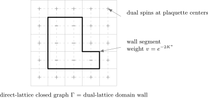
A closed graph on the direct lattice can be read as a domain wall for spins on the dual lattice. The high-temperature graph weight $v^{|\Gamma|}$ matches the dual low-temperature wall weight $e^{-2K^*|\Gamma|}$ when $e^{-2K^*}=v$.

Let us make this statement algebraic. From the high-temperature expansion derived previously,

$$Z_\Lambda(K) =2^{N_s}(\cosh K)^{N_b} \sum_{\Gamma:\partial\Gamma=0}(\tanh K)^{|\Gamma|},$$

where $\Gamma$ is a closed even subgraph, $N_s$ is the number of sites, and $N_b$ is the number of bonds.

Now consider an Ising model on this dual graph with coupling $K^*$. With the exterior dual spin fixed to $+$, its low-temperature expansion is

$$Z^+_{\Lambda^*}(K^*) =e^{K^*N_b}\sum_{\Gamma:\partial\Gamma=0}e^{-2K^*|\Gamma|}.$$

The same set of closed curves $\Gamma$ appears in both formulas. Therefore the two graphical sums are identical if

$$\boxed{e^{-2K^*}=\tanh K.}$$

With this identification,

$$Z_\Lambda(K) =2^{N_s}(\cosh K)^{N_b}e^{-K^*N_b} Z^+_{\Lambda^*}(K^*).$$

This is the cleanest finite-volume relation for a simply connected planar graph with matched boundary conventions. On a torus, high-temperature graphs have four possible $\mathbb Z_2$ winding parities, whereas domain walls of strictly periodic dual spins occupy only the homologically trivial sector. Consequently one periodic partition function does not map to itself: the exact duality is a linear combination of the four periodic/antiperiodic boundary sectors. Those distinctions matter for finite-size partition functions and torus CFT, even though they do not move the bulk singularity in the thermodynamic limit.

Coupling relation and the self-dual point

The dual coupling is

$$K^*=-{1\over2}\log(\tanh K).$$

The map exchanges weak and strong coupling:

$$K\ll1 \quad\Longrightarrow\quad K^*\gg1,$$

and

$$K\gg1 \quad\Longrightarrow\quad K^*\ll1.$$

So the disordered high-temperature phase of one model is described by the ordered low-temperature expansion of the dual model. That is the essential physics: the variables appropriate in one phase become nonlocal variables in the other phase.

It is often useful to write the duality relation symmetrically. Starting from

$$e^{-2K^*}=\tanh K,$$

we obtain

$$e^{2K^*}=\coth K.$$

Then

$$\sinh(2K^*) ={1\over2}\left(e^{2K^*}-e^{-2K^*}\right) ={1\over2}\left(\coth K-\tanh K\right).$$

Since

$$\coth K-\tanh K ={\cosh K\over\sinh K}-{\sinh K\over\cosh K} ={1\over\sinh K\cosh K} ={2\over\sinh(2K)},$$

we get

$$\boxed{\sinh(2K)\sinh(2K^*)=1.}$$

This form makes it obvious that duality is an involution: if $K$ maps to $K^*$, then $K^*$ maps back to $K$.

The self-dual point satisfies

$$K=K^*.$$

Equivalently,

$$\sinh^2(2K_c)=1.$$

For $K_c>0$,

$$\sinh(2K_c)=1.$$

Solving gives

$$\boxed{K_c={1\over2}\log(1+\sqrt2).}$$

Numerically,

$$K_c\approx0.4406867935, \qquad T_c={J\over K_c}\approx2.269185314\,J.$$

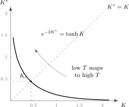
The Kramers–Wannier map $e^{-2K^*}=\tanh K$ exchanges high and low temperature. The square-lattice self-dual point lies at $K_c=K_c^*=\frac12\log(1+\sqrt2)$.

Duality by itself does not prove that the self-dual point is a critical point. It proves that if there is a unique transition separating the high- and low-temperature phases, then it must occur at the self-dual point. For the square-lattice Ising model, the exact solution confirms that this is indeed the critical point.

This caveat matters. A self-dual lattice model can have several transitions, or a first-order transition, or additional degrees of freedom that complicate the phase diagram. Duality is a structural constraint, not a substitute for the analysis of the thermodynamic limit.

Singular free energy and what duality really constrains

Let

$$f(K)=-\lim_{N_s\to\infty}{1\over N_s}\log Z_\Lambda(K)$$

be the dimensionless free-energy density. On the square lattice $N_b/N_s\to2$. The finite-volume duality relation implies, up to boundary and topological-sector details,

$$f(K)=f^+(K^*)-\log 2-2\log(\cosh K)+2K^*.$$

The last three terms are analytic for finite positive $K$. Thus the nonanalytic part of the free energy is mapped to the nonanalytic part at the dual coupling:

$$f_{\text{sing}}(K)=f^*_{\text{sing}}(K^*).$$

On a self-dual lattice, the original and dual thermodynamic systems are the same. Therefore singularities must be mapped to singularities under $K\mapsto K^*$. If the phase diagram has one critical point, it is forced to be fixed by duality.

The physical content is sharper than the formula may suggest. At small $K$, the original spins are disordered, but the dual model has large $K^*$ and is ordered. So the original spin variable is not mapped to a local dual spin variable. It is mapped to an object that detects dual domain walls. Conversely, the local dual spin is a disorder operator in the original variables. That is why the next pages introduce order and disorder fields rather than treating duality as a mere change of coupling.

Correlations and susceptibility

The Ising magnetization is

$$m={1\over N_s}\sum_i\langle\sigma_i\rangle,$$

or, more precisely in a phase with spontaneous symmetry breaking,

$$m_+=\lim_{h\to0^+}\lim_{N_s\to\infty}{1\over N_s}\sum_i\langle\sigma_i\rangle_h.$$

The connected two-point function is

$$G_c(i,j)=\langle\sigma_i\sigma_j\rangle-\langle\sigma_i\rangle\langle\sigma_j\rangle.$$

The zero-field susceptibility is the integrated connected correlator,

$$\chi=\sum_j G_c(i,j),$$

for a translation-invariant infinite lattice. It is also the derivative of the magnetization with respect to a uniform magnetic field:

$$\chi={\partial m\over\partial h}\bigg|_{h=0}.$$

This $\chi$ is dimensionless because $h=\beta H$. The susceptibility with respect to the physical field $H$ is $\chi_H=\beta\chi$.

At high temperature the correlation length is finite, and the sum converges. At a continuous transition the correlation length diverges, and the susceptibility diverges with it. One way to recognize the transition is therefore to look for the loss of stability of the $m=0$ solution. Mean-field theory turns this idea into a simple equation.

Exact local identity for one spin

Before making an approximation, let us write an exact identity. Allow a general symmetric coupling matrix $K_{ij}$ and external field $h_i$:

$$Z[h]=\sum_{\{\sigma\}}\exp\left( {1\over2}\sum_{i,j}K_{ij}\sigma_i\sigma_j+\sum_i h_i\sigma_i \right).$$

The factor $1/2$ avoids double counting when $K_{ij}=K_{ji}$, and we set $K_{ii}=0$. Define

$$B_i(\sigma)=h_i+\sum_j K_{ij}\sigma_j.$$

Holding all spins except $\sigma_i$ fixed, the part of the Boltzmann weight depending on $\sigma_i$ is

$$e^{\sigma_i B_i}.$$

The conditional average of $\sigma_i$ is therefore

$$\langle\sigma_i\rangle_{\text{conditional}} ={\sum_{\sigma_i=\pm1}\sigma_i e^{\sigma_iB_i} \over \sum_{\sigma_i=\pm1}e^{\sigma_iB_i}} ={2\sinh B_i\over2\cosh B_i} =\tanh B_i.$$

Averaging over the remaining spins gives the exact identity

$$\boxed{ \langle\sigma_i\rangle =\left\langle\tanh\left(h_i+\sum_jK_{ij}\sigma_j\right)\right\rangle. }$$

This formula is sometimes the safest way to remember what mean-field theory does. The exact equation averages a nonlinear function of fluctuating neighbors. Mean-field theory replaces the fluctuating neighbors by their average values.

Weiss mean-field equation

Define

$$m_i=\langle\sigma_i\rangle.$$

The Weiss approximation is

$$\left\langle\tanh\left(h_i+\sum_jK_{ij}\sigma_j\right)\right\rangle \approx \tanh\left(h_i+\sum_jK_{ij}m_j\right).$$

Thus

$$\boxed{ m_i=\tanh\left(h_i+\sum_jK_{ij}m_j\right). }$$

For a translation-invariant nearest-neighbor ferromagnet,

$$K_{ij}=K\quad\text{for nearest neighbors}, \qquad h_i=h, \qquad m_i=m,$$

and the sum over neighbors gives $zKm$. Hence

$$\boxed{m=\tanh(h+zKm).}$$

At $h=0$, the solution $m=0$ always exists. It is the only solution when $zK<1$. When $zK>1$, two additional nonzero solutions appear:

$$m=\pm m_0.$$

The mean-field critical coupling is therefore

$$\boxed{K_c^{\mathrm{MF}}={1\over z}.}$$

For the square lattice, $z=4$, so

$$K_c^{\mathrm{MF}}={1\over4}=0.25.$$

This is far from the exact square-lattice value $K_c\approx0.4406868$. Equivalently, mean-field theory predicts

$$T_c^{\mathrm{MF}}=4J,$$

whereas the exact answer is

$$T_c\approx2.269J.$$

The approximation overestimates the tendency to order because it suppresses fluctuations. A spin is assumed to see a smooth average environment, while in two dimensions domain walls fluctuate strongly.

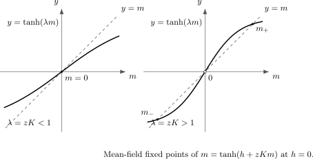
The mean-field equation at $h=0$ is the intersection of $y=m$ and $y=\tanh(\lambda m)$ with $\lambda=zK$. For $\lambda<1$, only $m=0$ exists. For $\lambda>1$, the symmetric solution becomes unstable and two stable symmetry-breaking solutions appear.

Variational free energy and Landau expansion

The same mean-field equation follows from the Gibbs variational principle. For any trial distribution $p$, the functional $\langle\beta H\rangle_p+\langle\log p\rangle_p$ bounds the exact dimensionless free energy from above. Restrict the trial states to the translation-invariant product distribution

$$p(\{\sigma\})=\prod_i {1+m\sigma_i\over2},$$

where $m$ is a trial magnetization. In this distribution,

$$\langle\sigma_i\rangle=m, \qquad \langle\sigma_i\sigma_j\rangle=m^2\quad(i\neq j).$$

The resulting dimensionless variational free energy per spin is

$$\varphi_{\mathrm{MF}}(m) =-{zK\over2}m^2-hm +{1+m\over2}\log{1+m\over2} +{1-m\over2}\log{1-m\over2}.$$

The first term is the average interaction energy. The factor $1/2$ avoids counting each bond twice. The last two terms are the entropy cost of biasing a two-state variable toward magnetization $m$.

The stationary condition is

$$0={\partial\varphi_{\mathrm{MF}}\over\partial m} =-zKm-h+{1\over2}\log{1+m\over1-m}.$$

Since

$${1\over2}\log{1+m\over1-m}=\operatorname{arctanh}m,$$

we get

$$\operatorname{arctanh}m=h+zKm,$$

or

$$m=\tanh(h+zKm).$$

Near $m=0$, expand the entropy term:

$${1+m\over2}\log{1+m\over2} +{1-m\over2}\log{1-m\over2} =-\log2+{1\over2}m^2+{1\over12}m^4+{1\over30}m^6+\cdots.$$

Therefore

$$\varphi_{\mathrm{MF}}(m) =-\log2 +{1\over2}(1-zK)m^2 +{1\over12}m^4 +{1\over30}m^6+\cdots -hm.$$

This is the first appearance of the Landau form. The coefficient of $m^2$ changes sign at $zK=1$, while the quartic term is positive. Thus a single minimum at $m=0$ becomes two minima at $m\neq0$.

At $h=0$ and $zK$ slightly above $1$, the stationary equation from the Landau expansion is

$$(1-zK)m+{1\over3}m^3+\cdots=0.$$

The nonzero solutions obey

$$m^2\approx3(zK-1).$$

Thus mean-field theory predicts the order-parameter critical exponent

$$m\sim (K-K_c^{\mathrm{MF}})^{1/2}.$$

In the usual notation this is

$$\beta_{\mathrm{mag}}^{\mathrm{MF}}={1\over2}.$$

The subscript “mag” is included to avoid confusing the critical exponent $\beta_{\mathrm{mag}}$ with the inverse temperature $\beta=1/T$.

Mean-field susceptibility

Differentiate the mean-field equation

$$m=\tanh(h+zKm)$$

with respect to $h$. Let

$$\chi={\partial m\over\partial h}.$$

Then

$$\chi=(1-m^2)(1+zK\chi).$$

Solving gives

$$\boxed{ \chi={1-m^2\over1-zK(1-m^2)}. }$$

In the disordered phase $m=0$, so

$$\chi={1\over1-zK}.$$

The susceptibility diverges as $K\to K_c^{\mathrm{MF}}$ from below:

$$\chi\sim {1\over K_c^{\mathrm{MF}}-K}.$$

Thus

$$\gamma_{\mathrm{MF}}=1.$$

At the critical point itself, set $zK=1$ and expand

$$m=\tanh(h+m)=h+m-{1\over3}(h+m)^3+\cdots.$$

For small $h$ and $m$, the leading balance is

$$h\sim {1\over3}m^3,$$

so

$$m\sim h^{1/3}, \qquad \delta_{\mathrm{MF}}=3.$$

These exponents are not exact for the two-dimensional Ising model. The exact values are

$$\beta_{\mathrm{mag}}={1\over8}, \qquad \gamma={7\over4}, \qquad \delta=15.$$

That disagreement is not a small numerical defect. It is the reason renormalization and conformal field theory enter the story. Mean-field theory captures the topology of the phase diagram, but not the long-distance fluctuation physics below the upper critical dimension.

Spatially varying mean field and correlation length

Mean-field theory also gives a first glimpse of how a mass term appears in continuum field theory. Linearize the inhomogeneous equation around $m_i=0$:

$$m_i=h_i+\sum_jK_{ij}m_j+O(m^3).$$

For a nearest-neighbor model on a $d$-dimensional hypercubic lattice,

$$\sum_jK_{ij}m_j =K\sum_{\mu=1}^d\left(m_{i+\hat\mu}+m_{i-\hat\mu}\right).$$

Fourier transforming gives

$$m(k)=h(k)+K(k)m(k),$$

where

$$K(k)=2K\sum_{\mu=1}^d\cos(k_\mu a).$$

Therefore the momentum-space susceptibility is

$$\chi(k)={m(k)\over h(k)}={1\over1-K(k)}.$$

At small momentum,

$$K(k)=2dK-Ka^2k^2+O(k^4)=zK-Ka^2k^2+O(k^4).$$

Thus

$$\chi(k)\approx{1\over(1-zK)+Ka^2k^2}.$$

This has the continuum form

$$\chi(k)\sim {1\over r+c k^2},$$

with

$$r=1-zK, \qquad c=Ka^2.$$

The correlation length is therefore

$$\xi^2={c\over r} ={Ka^2\over1-zK},$$

so

$$\xi\sim (K_c^{\mathrm{MF}}-K)^{-1/2}.$$

This is the mean-field correlation-length exponent

$$\nu_{\mathrm{MF}}={1\over2}.$$

More importantly, the denominator

$$r+c k^2$$

is exactly the structure that becomes the quadratic part of the continuum Landau–Ginzburg action. The parameter $r$ is the temperature-like relevant coupling. At criticality $r=0$, the long-wavelength field becomes massless.

What duality and mean field teach differently

Kramers–Wannier duality and mean-field theory are almost opposite tools.

Duality is exact, nonlocal, and dimension-specific. It reorganizes the partition function by changing variables from spins to walls, and from walls to dual spins. It sees the deep symmetry between high and low temperature. It knows the exact square-lattice critical point, assuming the uniqueness of the transition. But it does not by itself compute the critical exponents or the full correlation functions.

Mean-field theory is local, approximate, and broadly applicable. It does not know the exact critical point in two dimensions. It does not know the exact exponents. But it provides the first effective potential for an order parameter and the first continuum inverse propagator $r+c k^2$. Those are the seeds of the field theory developed in the next pages.

The clean mental picture is this:

$$\text{duality} \quad \text{finds better variables},$$

while

$$\text{mean field} \quad \text{finds a first saddle point}.$$

The continuum theory of critical phenomena will keep both ideas. We will introduce fields whose saddle points describe possible phases, then use fluctuations and renormalization to correct the mean-field picture. We will also keep looking for dual variables, because sometimes the natural long-distance degrees of freedom are not the microscopic spins.

Summary

The high-temperature Ising expansion counts closed graphs with weight $(\tanh K)^{|\Gamma|}$. The low-temperature expansion of the dual Ising model counts the same closed curves as domain walls with weight $e^{-2K^*|\Gamma|}$. Matching the weights gives

$$e^{-2K^*}=\tanh K,$$

or equivalently

$$\sinh(2K)\sinh(2K^*)=1.$$

For the square lattice, the self-dual coupling is

$$K_c={1\over2}\log(1+\sqrt2).$$

Assuming a unique transition, this is the critical point.

Mean-field theory starts from the exact identity

$$\langle\sigma_i\rangle =\left\langle\tanh\left(h_i+\sum_jK_{ij}\sigma_j\right)\right\rangle$$

and replaces neighboring spins by their averages. For a uniform nearest-neighbor system this gives

$$m=\tanh(h+zKm).$$

The symmetric solution becomes unstable at $zK=1$. The variational free energy has the Landau expansion

$$\varphi_{\mathrm{MF}}(m) =-\log2+{1\over2}(1-zK)m^2+{1\over12}m^4+\cdots-hm.$$

Mean-field theory predicts

$$\beta_{\mathrm{mag}}^{\mathrm{MF}}={1\over2}, \qquad \gamma_{\mathrm{MF}}=1, \qquad \delta_{\mathrm{MF}}=3, \qquad \nu_{\mathrm{MF}}={1\over2}.$$

These are not the two-dimensional Ising exponents, but the method points directly toward the continuum field theory of the order parameter.

Common pitfalls

Equating self-duality with criticality. The self-dual point need not be critical in every self-dual model. For the square-lattice Ising ferromagnet, uniqueness of the transition and the exact solution place the singularity at the fixed point.

Identifying the dual spin with the original spin. Kramers–Wannier duality maps a local spin description in one phase to a nonlocal disorder description in the other. This distinction becomes essential when defining disorder operators.

Ignoring topology in finite volume. On a torus, a periodic partition function mixes with periodic/antiperiodic sectors under duality. The simple one-to-one contour formula is exact for the matched planar boundary conditions stated above, not for a single periodic sector by itself.

Trusting mean field quantitatively in two dimensions. Mean-field theory suppresses domain-wall and long-wavelength fluctuations. Its value here is structural: it introduces an order-parameter potential and the mass term that later enter the continuum theory.

Losing the field and exponent conventions. Here $h=\beta H$ is dimensionless, so differentiation with respect to the physical field supplies an extra factor of $\beta$. The inverse temperature $\beta=1/T$ is also distinct from the magnetization exponent, written as $\beta_{\mathrm{mag}}$.

Exercises

Exercise 1

Show that the Kramers–Wannier relation

$$e^{-2K^*}=\tanh K$$

is equivalent to

$$\sinh(2K)\sinh(2K^*)=1.$$

Then solve the self-duality equation $K=K^*$.

Solution

From

$$e^{-2K^*}=\tanh K,$$

we have

$$e^{2K^*}=\coth K.$$

Therefore

$$\sinh(2K^*) ={1\over2}(e^{2K^*}-e^{-2K^*}) ={1\over2}(\coth K-\tanh K).$$

Using

$$\coth K-\tanh K ={\cosh^2K-\sinh^2K\over\sinh K\cosh K} ={1\over\sinh K\cosh K} ={2\over\sinh(2K)},$$

we obtain

$$\sinh(2K^*)={1\over\sinh(2K)}.$$

Thus

$$\sinh(2K)\sinh(2K^*)=1.$$

At the self-dual point, $K=K^*$, so

$$\sinh^2(2K_c)=1.$$

For positive coupling,

$$\sinh(2K_c)=1.$$

Thus

$$e^{2K_c}-e^{-2K_c}=2.$$

Let $x=e^{2K_c}$. Then

$$x-{1\over x}=2,$$

so

$$x^2-2x-1=0.$$

The positive solution is

$$x=1+\sqrt2.$$

Therefore

$$K_c={1\over2}\log(1+\sqrt2).$$

Exercise 2

Derive the exact identity

$$\langle\sigma_i\rangle =\left\langle\tanh\left(h_i+\sum_jK_{ij}\sigma_j\right)\right\rangle$$

for the Ising model with general couplings $K_{ij}=K_{ji}$ and fields $h_i$. Then state precisely where the mean-field approximation enters.

Solution

Write the Boltzmann weight as

$$\exp\left({1\over2}\sum_{j,k}K_{jk}\sigma_j\sigma_k+\sum_jh_j\sigma_j\right).$$

Fix all spins except $\sigma_i$. The dependence on $\sigma_i$ is

$$\exp\left[\sigma_i\left(h_i+\sum_jK_{ij}\sigma_j\right)\right].$$

Define

$$B_i=h_i+\sum_jK_{ij}\sigma_j.$$

The conditional average is

$${\sum_{\sigma_i=\pm1}\sigma_i e^{\sigma_iB_i} \over \sum_{\sigma_i=\pm1}e^{\sigma_iB_i}} ={e^{B_i}-e^{-B_i}\over e^{B_i}+e^{-B_i}} =\tanh B_i.$$

Averaging over the remaining spins gives

$$\langle\sigma_i\rangle =\langle\tanh B_i\rangle.$$

Mean-field theory replaces the fluctuating neighboring spins inside $B_i$ by their averages:

$$\sigma_j\mapsto m_j=\langle\sigma_j\rangle.$$

It also replaces the average of the nonlinear function by the function of the averaged argument:

$$\left\langle\tanh\left(h_i+\sum_jK_{ij}\sigma_j\right)\right\rangle \approx \tanh\left(h_i+\sum_jK_{ij}m_j\right).$$

Thus

$$m_i=\tanh\left(h_i+\sum_jK_{ij}m_j\right).$$

Exercise 3

For the uniform mean-field equation at zero field,

$$m=\tanh(zKm),$$

show that a nonzero solution appears when $zK>1$. Near the mean-field critical point, derive

$$m\approx\pm\sqrt{3(zK-1)}.$$

Solution

Expand the right-hand side for small $m$:

$$\tanh(zKm)=zKm-{1\over3}(zKm)^3+O(m^5).$$

The self-consistency equation becomes

$$m=zKm-{1\over3}(zK)^3m^3+O(m^5).$$

Move all terms to one side:

$$(1-zK)m+{1\over3}(zK)^3m^3+O(m^5)=0.$$

One solution is $m=0$. For a nonzero solution, divide by $m$:

$$1-zK+{1\over3}(zK)^3m^2+O(m^4)=0.$$

Thus

$$m^2\approx {3(zK-1)\over (zK)^3}.$$

Very close to the critical point $zK=1$, the denominator may be replaced by $1$ at leading order, giving

$$m\approx\pm\sqrt{3(zK-1)}.$$

A real nonzero solution exists only for $zK>1$.

Exercise 4

Linearize the inhomogeneous mean-field equation on a $d$-dimensional hypercubic lattice and show that the susceptibility has the small-momentum form

$$\chi(k)\approx {1\over (1-zK)+Ka^2k^2}.$$

Extract the mean-field correlation length.

Solution

The inhomogeneous mean-field equation is

$$m_i=\tanh\left(h_i+K\sum_{\mu=1}^d(m_{i+\hat\mu}+m_{i-\hat\mu})\right).$$

In the disordered phase and for small field, linearize $\tanh x\approx x$:

$$m_i=h_i+K\sum_{\mu=1}^d(m_{i+\hat\mu}+m_{i-\hat\mu}).$$

Fourier transform with lattice spacing $a$:

$$m_i=\int_k e^{ik\cdot x_i}m(k), \qquad h_i=\int_k e^{ik\cdot x_i}h(k).$$

Then

$$\sum_{\mu=1}^d(m_{i+\hat\mu}+m_{i-\hat\mu}) \mapsto 2\sum_{\mu=1}^d\cos(k_\mu a)m(k).$$

Therefore

$$m(k)=h(k)+2K\sum_{\mu=1}^d\cos(k_\mu a)m(k),$$

so

$$\chi(k)={m(k)\over h(k)} ={1\over1-2K\sum_\mu\cos(k_\mu a)}.$$

At small $k$,

$$\cos(k_\mu a)=1-{1\over2}k_\mu^2a^2+O(k^4),$$

hence

$$2K\sum_{\mu=1}^d\cos(k_\mu a) =2dK-Ka^2k^2+O(k^4).$$

Since $z=2d$,

$$\chi(k)\approx{1\over(1-zK)+Ka^2k^2}.$$

Writing this as

$$\chi(k)\approx {1\over r+c k^2}$$

with

$$r=1-zK, \qquad c=Ka^2,$$

the correlation length is

$$\xi^2={c\over r}={Ka^2\over1-zK}.$$

Thus

$$\xi\sim(K_c^{\mathrm{MF}}-K)^{-1/2}, \qquad \nu_{\mathrm{MF}}={1\over2}.$$

References

• Hendrik A. Kramers and Gregory H. Wannier, “Statistics of the Two-Dimensional Ferromagnet. Part I,” Physical Review 60 (1941), 252–262.
• Lars Onsager, “Crystal Statistics. I. A Two-Dimensional Model with an Order-Disorder Transition,” Physical Review 65 (1944), 117–149.

Further reading

• Rodney J. Baxter, Exactly Solved Models in Statistical Mechanics, Academic Press, 1982.
• Nigel Goldenfeld, Lectures on Phase Transitions and the Renormalization Group, Addison-Wesley, 1992.
• Alexander M. Polyakov, Gauge Fields and Strings, Harwood Academic Publishers, 1987, Chapters 1 and 3.
• Jean Zinn-Justin, Quantum Field Theory and Critical Phenomena, 5th ed., Oxford University Press, 2021, Chapters 14–16.