Schwarzian Derivative and the Virasoro Algebra

The central pole in the stress-tensor OPE has a finite geometric consequence. On the Euclidean plane, the holomorphic stress tensor transforms with an additive Schwarzian derivative proportional to its central charge $c$. At nonzero $c$ it is therefore not a primary field under arbitrary local conformal maps. We derive the coordinate-change law on invertible patches, then use it to relate the plane identity vacuum to cylinder energy and radial adjoints.

This is one of the most compact places where the whole structure of two-dimensional conformal field theory shows itself. The same coefficient $c$ appears in three equivalent ways:

$$T(z)T(w) \sim {c/2\over (z-w)^4}+{2T(w)\over (z-w)^2}+{\partial T(w)\over z-w},$$ $$T_z(z)=\left({df\over dz}\right)^2T_w(f(z))+{c\over 12}\{f,z\},$$

and

$$[L_n,L_m]=(n-m)L_{n+m}+{c\over 12}n(n^2-1)\delta_{n+m,0}.$$

The first is local short-distance data, the second is the finite coordinate-transformation law, and the third is the operator algebra of infinitesimal conformal transformations. Their common normalization relates short-distance products, coordinate changes, and radial quantization.

Required background. Lesson 23 supplies the $T T$ OPE, the mode convention, and the central extension used below.

The stress tensor is almost primary

We work in one holomorphic sector; the barred sector has the corresponding formulas. The mode convention is

$$L_n={1\over 2\pi i}\oint_0 dz\,z^{n+1}T(z), \qquad T(z)=\sum_{n\in\mathbb Z}L_nz^{-n-2}.$$

Contours are counterclockwise, and products are radially ordered. A contour deformation is made within a region where the stress tensor and its chosen weight are single-valued and no other singularity is crossed. The positive active Ward operation is

$$\delta_\epsilon\mathcal O(w) ={1\over2\pi i}\oint_w dz\,\epsilon(z)T(z)\mathcal O(w).$$

For a primary of weight $h$ this gives $\delta_\epsilon\mathcal O=\epsilon\partial\mathcal O+h\epsilon'\mathcal O$. The contour around $w$ is a local operation; it is not automatically the origin-centered mode acting on a field. Lesson 22’s mode contours distinguish these operations. We keep this positive sign throughout and explicitly invert the finite coordinate formula below.

A primary field of holomorphic weight $h$ has OPE

$$T(z)\mathcal O(w) \sim {h\mathcal O(w)\over (z-w)^2} +{\partial\mathcal O(w)\over z-w}.$$

Multiplying by $\epsilon(z)$ and taking the residue at $z=w$ gives

$$\delta_\epsilon\mathcal O(w)=\epsilon(w)\partial\mathcal O(w)+h\partial\epsilon(w)\mathcal O(w).$$

If the stress tensor were an ordinary primary of weight $2$, we would have only

$$\delta_\epsilon T=\epsilon\partial T+2(\partial\epsilon)T.$$

But the stress tensor has the OPE with itself

$$T(z)T(w) \sim {c/2\over (z-w)^4} +{2T(w)\over (z-w)^2} +{\partial T(w)\over z-w}.$$

The fourth-order pole is a c-number singularity proportional to the identity, rather than to $T$ or one of its descendants. It is the local shadow of the central extension. Applying the contour prescription gives

$$\delta_\epsilon T(w) ={1\over 2\pi i}\oint_w dz\,\epsilon(z)T(z)T(w).$$

The weight-$2$ terms are immediate. For the central term, use

$${1\over 2\pi i}\oint_w dz\,{\epsilon(z)\over (z-w)^4} ={1\over 3!}\partial_w^3\epsilon(w).$$

Therefore

$$\boxed{ \delta_\epsilon T =\epsilon\partial T+2(\partial\epsilon)T+{c\over 12}\partial^3\epsilon. }$$

The stress tensor is therefore not a Virasoro primary when $c\ne0$. It is quasi-primary under the global Möbius subgroup, for which the inhomogeneous term vanishes, but a general local conformal transformation acts on it as a weight-$2$ field plus the third-derivative term.

A useful immediate check is the global conformal subgroup. On the Riemann sphere, the globally defined holomorphic vector fields are

$$\epsilon(z)=a_0+a_1z+a_2z^2.$$

For these transformations,

$$\partial^3\epsilon=0.$$

Thus translations, dilatations/rotations, and special conformal transformations do not see the central term. The anomaly appears only for genuinely local conformal transformations.

The Schwarzian derivative and finite coordinate changes

Let $w=f(z)$ be a holomorphic coordinate change with $f'(z)\ne0$ on the patch in use. Where we use $f^{-1}$, restrict to a one-to-one coordinate patch. The formulas are local: maps with critical points, singularities, or multiple sheets require separate charts or additional data.

Define

$$S(f;z)\equiv\{f,z\} ={f'''(z)\over f'(z)} -{3\over2}\left({f''(z)\over f'(z)}\right)^2.$$

The stress tensors in the two coordinates satisfy

$$T_z(z)=(f'(z))^2T_w(f(z))+{c\over12}S(f;z).$$

The first term pulls back a quadratic differential; the second is inhomogeneous. When $c\ne0$, the rescaled quantity $12T/c$ has the standard projective-connection transformation law. When $c=0$, $T$ transforms as a quadratic differential.

To keep the direction explicit, define the affine pullback of a fixed reference field by

$$A_f[T](z)=(f'(z))^2T(f(z))+{c\over12}S(f;z).$$

The passive relation is $T_z=A_f[T_w]$. Solving for the other coordinate gives

$$\begin{aligned} T_w(w) &=\left. {T_z(z)-(c/12)S(f;z)\over(f'(z))^2} \right|_{z=f^{-1}(w)} \\ &=((f^{-1})'(w))^2T_z(f^{-1}(w)) +{c\over12}S(f^{-1};w). \end{aligned}$$

Equivalently, $T_w=A_{f^{-1}}[T_z]$. These are inverse descriptions of the same coordinate relation. In the active pullback $A_f[T]$, the reference field $T$ is held fixed; its inverse operation is $A_{f^{-1}}[T]$. One must specify that direction before comparing infinitesimal signs.

For a controlled expansion, fix a holomorphic profile $\epsilon$ and let $f_t(z)=z+t\epsilon(z)$. On a compact subpatch with bounded derivatives, take $t$ small enough that $\lvert t\epsilon'\rvert<1$ and use an invertible restriction. In matrix elements away from other insertions,

$$\begin{aligned} (f_t')^2T(f_t) &=T+t(\epsilon\partial T+2\epsilon'T)+O(t^2),\\ S(f_t;z)&=t\epsilon'''+O(t^2),\\ A_{f_t}[T]-T &=t\left(\epsilon\partial T+2\epsilon'T +{c\over12}\epsilon'''\right)+O(t^2). \end{aligned}$$

This is precisely the positive contour variation derived above. Since $f_t^{-1}(z)=z-t\epsilon(z)+O(t^2)$, its active pullback has the negative variation. Di Francesco, Mathieu, and Sénéchal use that negative infinitesimal convention; solving their finite equation for the original tensor gives our positive pullback. See Di Francesco, Mathieu, and Sénéchal 1997, §5.4.1, pp.136–138, Eqs.(5.123)–(5.136).

Why successive maps agree

The Schwarzian vanishes for a Möbius map $f(z)=(az+b)/(c_{\mathrm M}z+d)$ with $ad-bc_{\mathrm M}\ne0$, on a chart where its denominator is nonzero. Its derivatives cancel explicitly, as in Exercise 2. Such maps therefore act on $T$ without the inhomogeneous term.

The composition law can be derived without guessing:

$$u_f={f''\over f'},\qquad S(f)=u_f'-{1\over2}u_f^2, \qquad u_{f\circ g}=(u_f\circ g)g'+u_g.$$

On differentiating and subtracting half the square, the cross term cancels because $u_g=g''/g'$. Thus

$$\begin{aligned} S(f\circ g;z) &=(g')^2\left(u_f'-{1\over2}u_f^2\right)\!\circ g +\left(u_g'-{1\over2}u_g^2\right)\\ &=(g')^2S(f;g(z))+S(g;z). \end{aligned}$$

Consequently $A_g[A_f[T]]=A_{f\circ g}[T]$: pullbacks compose in the reverse operator order to coordinate maps. Setting $g=f^{-1}$ gives the inverse identity used above. These formulas agree with Di Francesco, Mathieu, and Sénéchal 1997, §5.4.1, p.137, Eqs.(5.129)–(5.132).

This also explains how the infinitesimal law integrates locally. Let $f_t$ be a smooth path of invertible holomorphic maps with $f_0(z)=z$, remaining on suitable patches. Define the right-composition velocity $\epsilon_t(z)=\dot f_t(z)/f_t'(z)$. Then

$$f_{t+dt}=f_t\circ(\mathrm{id}+dt\,\epsilon_t)+O(dt^2).$$

Writing $T_t=A_{f_t}[T]$ and using the composition law gives

$$\dot T_t =\epsilon_t\partial T_t+2\epsilon_t'T_t +{c\over12}\epsilon_t'''.$$

The finite pullback therefore solves the Ward transport with its specified initial field. Locally this first-order linear transport fixes the solution along characteristics, as long as the maps and matrix elements remain regular. This is a coordinate-patch statement; it does not establish a global unitary representation of every conformal transformation.

Which cocycle appears here?

The Schwarzian composition law is a cocycle with values in weight-two fields: the old inhomogeneous term acquires the Jacobian squared when transported, and the next map contributes its own term. It makes the affine action on $T$ consistent.

A projective action on states instead has a two-argument phase, for example $U(g_1)U(g_2)=e^{i\alpha(g_1,g_2)}U(g_1g_2)$. Its phase cocycle is not literally the one-argument Schwarzian. The infinitesimal central extension is represented here by the TT OPE and the Virasoro commutator; the finite affine law does not by itself prove that a state-space action has been globally integrated. The same coefficient $c$ fixes both the infinitesimal anomaly and the Schwarzian term.

Virasoro algebra from the TT OPE

The following calculation also checks the normalization used in Lesson 23. The difference of radial orderings produces a local contour about the second stress insertion, followed by an origin contour. This construction is explained in Di Francesco, Mathieu, and Sénéchal 1997, §6.1.2, pp.154–155, Eqs.(6.13)–(6.18), and §6.2.1, pp.155–157, Eqs.(6.21)–(6.25). Define

$$L_n={1\over2\pi i}\oint_0 dz\,z^{n+1}T(z).$$

The commutator is computed by radial ordering: one contour surrounds the other, and the difference is the contour that picks up the singularity of $T(z)T(w)$ at $z=w$.

Using only the singular part of the OPE,

$$[L_n,L_m] ={1\over2\pi i}\oint_0 dw\,w^{m+1} \operatorname{Res}_{z=w}\left[z^{n+1}T(z)T(w)\right].$$

The double-pole term gives

$$\operatorname{Res}_{z=w}\left[z^{n+1}{2T(w)\over (z-w)^2}\right] =2(n+1)w^nT(w).$$

The simple-pole term gives

$$\operatorname{Res}_{z=w}\left[z^{n+1}{\partial T(w)\over z-w}\right] =w^{n+1}\partial T(w).$$

After multiplying by $w^{m+1}$ and integrating, the derivative term is integrated by parts:

$${1\over2\pi i}\oint dw\,w^{m+n+2}\partial T(w) =-(m+n+2)L_{m+n}.$$

Together these two operator terms give

$$\left[2(n+1)-(m+n+2)\right]L_{m+n}=(n-m)L_{m+n}.$$

The central pole gives

$$\operatorname{Res}_{z=w}\left[z^{n+1}{c/2\over (z-w)^4}\right] ={c\over2}{1\over3!}\partial_w^3w^{n+1} ={c\over12}n(n^2-1)w^{n-2}.$$

Multiplying by $w^{m+1}$ and taking the $w$ residue yields

$${c\over12}n(n^2-1)\delta_{n+m,0}.$$

Therefore

$$\boxed{ [L_n,L_m]=(n-m)L_{n+m}+{c\over12}n(n^2-1)\delta_{n+m,0}. }$$

This is the Virasoro algebra. If $c=0$, it reduces to the Witt algebra of holomorphic vector fields

$$\ell_n=-z^{n+1}\partial_z, \qquad [\ell_n,\ell_m]=(n-m)\ell_{n+m}.$$

In this quantum stress-tensor realization, the fourth-order OPE pole fixes the central extension of the Witt algebra. The algebraic derivation does not require reflection positivity.

Global conformal transformations and the missing central term

The modes

$$L_{-1},\quad L_0,\quad L_1$$

generate the globally defined holomorphic transformations on the sphere:

$$1,\quad z,\quad z^2.$$

The central term is proportional to

$$n(n^2-1),$$

so it vanishes for $n=-1,0,1$. Hence

$$[L_0,L_{-1}]=L_{-1}, \qquad [L_0,L_1]=-L_1, \qquad [L_1,L_{-1}]=2L_0.$$

This is the Lie algebra of the global conformal group. The infinitesimal inhomogeneous term is proportional to the third derivative of the vector field. It vanishes for the three global polynomial generators. A particular mode commutator also needs opposite mode indices for a nonzero central term; being outside the global subalgebra is not sufficient for every bracket to have one.

This distinction is conceptually important. Global conformal invariance fixes two- and three-point functions and constrains four-point functions. Local conformal invariance, through the full Virasoro algebra, organizes an infinite tower of descendants and gives much stronger constraints. Minimal models owe their solvability to this enhancement.

A useful consistency check is the action of the global generators on the first descendant of a primary state. If $|h\rangle$ is primary, then

$$[L_1,L_{-1}]|h\rangle=L_1L_{-1}|h\rangle=2h|h\rangle.$$

The same result follows directly from the OPE. Differentiate

$$T(z)\phi(w) \sim {h\phi(w)\over(z-w)^2} +{\partial\phi(w)\over z-w}$$

with respect to $w$ and set $w=0$:

$$T(z)\,\partial\phi(0) \sim {2h\phi(0)\over z^3} +{(h+1)\partial\phi(0)\over z^2} +{\partial^2\phi(0)\over z}.$$

The coefficient of $z^{-3}$ is $2h\phi(0)$. In the local descendant notation of Lesson 22 it is $(L_1^{(0)}L_{-1}^{(0)}\phi)(0)$; under the state–operator map it corresponds to $L_1L_{-1}|h\rangle=2h|h\rangle$. This is the level-one version of the contour derivation.

Plane-to-cylinder map and Casimir energy

Use the cylinder coordinate $w=\tau+i\theta$, with $\theta\sim\theta+2\pi$, and the map

$$z=e^w.$$

Its image is the punctured plane; a logarithmic inverse requires a branch on a coordinate patch. The plane–cylinder geometry in Lesson 22 shows radial time and the angular identification. Here the new ingredient is the Schwarzian:

$$S(e^w;w) ={z'''\over z'}-{3\over2}\left({z''\over z'}\right)^2 =1-{3\over2}=-{1\over2}.$$

Therefore

$$T_{\mathrm{cyl}}(w)=z^2T_{\mathrm{pl}}(z)-{c\over24}.$$

In the state obtained by transporting the normalized plane identity vacuum, $\langle T_{\mathrm{pl}}\rangle=0$, so $\langle T_{\mathrm{cyl}}\rangle=-c/24$. This is a statement about that state. It does not identify the lowest energy in every possible boundary-condition or operator sector. The coordinate transformation and plane-vacuum expectation follow Di Francesco, Mathieu, and Sénéchal 1997, §5.4.2, pp.138–139, Eqs.(5.137)–(5.139).

For a nonchiral theory with $c=\bar c$, velocity one, and circumference $L$, the energy and momentum operators are

$$H={2\pi\over L}\left(L_0+\bar L_0-{c\over12}\right), \qquad P={2\pi\over L}(L_0-\bar L_0).$$

An eigenstate of weights $h,\bar h$ thus has

$$E={2\pi\over L}\left(h+\bar h-{c\over12}\right), \qquad P={2\pi\over L}(h-\bar h).$$

Descendants are included by using their shifted eigenvalues. If the chosen sector has an attained lowest state of weights $h_0,\bar h_0$, then

$$E_0={2\pi\over L}\left(h_0+\bar h_0-{c\over12}\right).$$

When the lowest total weight satisfies $h_0+\bar h_0=0$, this reduces to $E_0=-\pi c/(6L)$. The same central charge that appears in the local fourth-order pole supplies the universal energy offset; the spectrum of allowed states determines the rest.

Reflection positivity and adjoints

For the positivity argument, assume vacuum Euclidean correlators with an antilinear reflection/adjunction operation $\Theta$ satisfying

$$\langle(\Theta A)A\rangle\ge0$$

for admissible smeared bosonic products $A$ supported on one side of the reflection surface. This is a condition on the correlation functions, not a claim that every functional-integral representation has a positive measure. For a scalar insertion, reflection reverses Euclidean time and takes the field adjoint; only for a Hermitian scalar does this reduce to the same field at the reflected point. The operation also conjugates coefficients and reverses operator order.

In radial quantization, $\tau=\log|z|$. Reflection about $\tau=0$ is

$$z=r e^{i\theta}\longmapsto {1\over\bar z} =r^{-1}e^{i\theta}.$$

Inspect the unchanged angle and reciprocal radii in the figure. The insertion points lie on opposite sides of the unit quantization circle, and their logarithmic times have opposite signs.

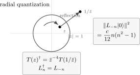
The exact example uses $\theta=\pi/6$ and $r=1/2$ and $2$. Reflection in the unit quantization circle sends $z$ to $1/\bar z$ and $\tau=\log r$ to $-\tau$. This geometry identifies reflected insertions; reflection positivity is a separate hypothesis on their correlation functions.

The holomorphic inversion has zero Schwarzian, so the stress tensor’s radial adjoint has the weight-two factor even though $T$ is not primary under a general local map:

$$T(z)^\dagger=\bar z^{-4}T\left({1\over\bar z}\right).$$

Using the Laurent expansion on both sides gives

$$\sum_n\bar z^{-n-2}L_n^\dagger =\sum_n\bar z^{n-2}L_n =\sum_n\bar z^{-n-2}L_{-n},$$

hence $L_n^\dagger=L_{-n}$. The radial adjunction and mode convention are developed in Di Francesco, Mathieu, and Sénéchal 1997, §6.1.1, pp.151–153, Eqs.(6.1), (6.4), (6.7)–(6.10).

Take the identity vacuum with $\langle0|0\rangle=1$ and regular $T(z)|0\rangle$ at the origin. The absence of negative powers in its Laurent expansion gives

$$L_n|0\rangle=0\qquad(n\ge-1).$$

This full condition follows from regularity; global invariance alone only tests the three global generators. For $n\ge2$,

$$\begin{aligned} \|L_{-n}|0\rangle\|^2 &=\langle0|L_nL_{-n}|0\rangle\\ &=\langle0|[L_n,L_{-n}]|0\rangle ={c\over12}n(n^2-1). \end{aligned}$$

Reflection positivity therefore requires $c\ge0$. This is a necessary condition, not a classification of unitary representations. The algebra itself may be studied without these positivity assumptions. The regular-vacuum condition and descendant norm agree with Di Francesco, Mathieu, and Sénéchal 1997, §6.2.2, p.157, Eqs.(6.26)–(6.27), and §7.2.1, p.205, Eq.(7.19).

Summary

The central charge can be read in several mutually reinforcing ways.

The local OPE statement is

$$T(z)T(w) \sim {c/2\over (z-w)^4} +{2T(w)\over (z-w)^2} +{\partial T(w)\over z-w}.$$

The infinitesimal transformation statement is

$$\delta_\epsilon T=\epsilon\partial T+2(\partial\epsilon)T+{c\over12}\partial^3\epsilon.$$

The finite geometric statement is

$$T_z(z)=(f'(z))^2T_w(f(z))+{c\over12}\{f,z\}.$$

The mode-algebra statement is

$$[L_n,L_m]=(n-m)L_{n+m}+{c\over12}n(n^2-1)\delta_{n+m,0}.$$

The physical finite-size statement is that the Schwarzian shifts the cylinder Hamiltonian. Identifying its ground-state energy additionally requires the lowest weights in the chosen sector. The TT pole, affine coordinate transformation, and mode central term share one normalization.

Common pitfalls

At nonzero central charge, the stress tensor is not a primary field under arbitrary local conformal maps. It is primary-like under the global Möbius group because the Schwarzian vanishes there, but under general holomorphic maps it has an additive term.

The affine pullback $A_f[T]$ gives the positive contour variation while $A_{f^{-1}}[T]$ gives its negative near the identity. Solving a passive coordinate relation for the other tensor reverses the Jacobian and the inhomogeneous term together. Keep the held-fixed reference field explicit.

The central term in the Virasoro algebra is not optional once the $T T$ OPE has a fourth-order pole. Removing it would destroy the Ward identities and the plane–cylinder Casimir shift.

The global conformal algebra is not the whole story in two dimensions. The modes $L_{-1},L_0,L_1$ form an $sl(2)$ subalgebra, but the local stress-tensor algebra contains all $L_n$ and is much more restrictive.

Exercises

Exercise 1: Infinitesimal stress-tensor anomaly

Use a counterclockwise local contour on a patch where the test function is holomorphic and no other insertion is enclosed. Use the OPE

$$T(z)T(w) \sim {c/2\over (z-w)^4}+{2T(w)\over (z-w)^2}+{\partial T(w)\over z-w}$$

to derive

$$\delta_\epsilon T=\epsilon\partial T+2(\partial\epsilon)T+{c\over12}\partial^3\epsilon.$$

Solution

By the Ward-identity contour prescription,

$$\delta_\epsilon T(w) ={1\over2\pi i}\oint_w dz\,\epsilon(z)T(z)T(w).$$

Only singular terms contribute. The simple pole gives

$${1\over2\pi i}\oint_w dz\,\epsilon(z){\partial T(w)\over z-w} =\epsilon(w)\partial T(w).$$

The double pole gives

$${1\over2\pi i}\oint_w dz\,\epsilon(z){2T(w)\over (z-w)^2} =2\partial\epsilon(w)T(w).$$

The fourth-order pole gives

$${c\over2}{1\over2\pi i}\oint_w dz\,{\epsilon(z)\over (z-w)^4} ={c\over2}{1\over3!}\partial^3\epsilon(w) ={c\over12}\partial^3\epsilon(w).$$

Adding the three pieces gives the result.

Exercise 2: Möbius maps have vanishing Schwarzian

Work on a coordinate patch with $cz+d\ne0$. In this exercise, $c$ in the matrix entries is unrelated to the central charge. Show that the Schwarzian derivative vanishes for

$$f(z)={az+b\over cz+d}, \qquad ad-bc\ne0.$$

Solution

Let $D=ad-bc$. Then

$$f'(z)={D\over (cz+d)^2}, \qquad f''(z)=-{2cD\over (cz+d)^3}, \qquad f'''(z)={6c^2D\over (cz+d)^4}.$$

Hence

$${f'''\over f'}={6c^2\over (cz+d)^2}, \qquad \left({f''\over f'}\right)^2={4c^2\over (cz+d)^2}.$$

Therefore

$$\{f,z\} ={6c^2\over (cz+d)^2} -{3\over2}{4c^2\over (cz+d)^2}=0.$$

This is why the stress tensor transforms as an ordinary weight-$2$ field under global conformal transformations.

Exercise 3: Central term from the fourth-order pole

Starting from the $T T$ OPE and the mode definition

$$L_n={1\over2\pi i}\oint dz\,z^{n+1}T(z),$$

derive the central term in $[L_n,L_m]$. Use counterclockwise contours: after taking the difference of radial orderings, first take the local $z$ residue about $w$ with weight $z^{n+1}$, then the origin-centered $w$ contour. No other singularity is crossed in the deformation.

Solution

The central term comes only from

$${c/2\over (z-w)^4}.$$

In the contour computation,

$$[L_n,L_m]_{\mathrm{cent}} ={1\over2\pi i}\oint_0 dw\,w^{m+1} \operatorname{Res}_{z=w}\left(z^{n+1}{c/2\over (z-w)^4}\right).$$

The residue is

$${c\over2}{1\over3!}\partial_w^3w^{n+1} ={c\over12}n(n^2-1)w^{n-2}.$$

Thus

$$[L_n,L_m]_{\mathrm{cent}} ={c\over12}n(n^2-1){1\over2\pi i}\oint_0dw\,w^{m+n-1} ={c\over12}n(n^2-1)\delta_{m+n,0}.$$

Exercise 4: Plane-to-cylinder Casimir shift

Compute the Schwarzian derivative of $z=e^w$ on the cylinder of circumference $2\pi$. In the state transported from the normalized plane identity vacuum, assume $\langle T_{\mathrm{pl}}(z)\rangle=0$ and find the holomorphic cylinder stress expectation. No claim about a different sector’s lowest state is intended.

Solution

For $z=e^w$,

$$z'=z, \qquad z''=z, \qquad z'''=z.$$

Therefore

$$\{e^w,w\} ={z'''\over z'}-{3\over2}\left({z''\over z'}\right)^2 =1-{3\over2}=-{1\over2}.$$

The finite transformation law gives

$$T_{\mathrm{cyl}}(w)=z^2T_{\mathrm{pl}}(z)+{c\over12}\{e^w,w\} =z^2T_{\mathrm{pl}}(z)-{c\over24}.$$

Taking the plane vacuum expectation value gives

$$\langle T_{\mathrm{cyl}}\rangle=-{c\over24}.$$

The antiholomorphic sector gives the analogous shift $-\bar c/24$.

Exercise 5: Positivity of the stress-tensor state

Use the Virasoro algebra to compute $[L_2,L_{-2}]$. Assume the identity vacuum has unit norm, regular $T(z)|0\rangle$ at the origin, and $L_n^\dagger=L_{-n}$. Thus $L_n|0\rangle=0$ for $n\ge-1$. Compute the norm of $L_{-2}|0\rangle$.

Solution

The Virasoro algebra gives

$$[L_2,L_{-2}] =(2-(-2))L_0+{c\over12}2(2^2-1) =4L_0+{c\over2}.$$

The norm is

$$\langle0|L_2L_{-2}|0\rangle =\langle0|[L_2,L_{-2}]|0\rangle,$$

because $L_2|0\rangle=0$ and $\langle0|L_{-2}=0$ by conjugation. Since $L_0|0\rangle=0$,

$$\langle0|L_2L_{-2}|0\rangle={c\over2}.$$

In a unitary theory this norm is nonnegative, so this calculation gives the simple necessary condition $c\ge0$.

References

• Di Francesco, Philippe, Pierre Mathieu, and David Sénéchal. Conformal Field Theory. Graduate Texts in Contemporary Physics. New York: Springer, 1997. DOI.

Further reading

• A. A. Belavin, A. M. Polyakov, and A. B. Zamolodchikov, “Infinite conformal symmetry in two-dimensional quantum field theory,” Nuclear Physics B 241 (1984) 333–380.
• P. Ginsparg, “Applied Conformal Field Theory,” in Fields, Strings and Critical Phenomena, Les Houches Session XLIX, edited by E. Brézin and J. Zinn-Justin (Elsevier, 1989), pp. 1–168.
• J. Polchinski, String Theory, Volume 1 (Cambridge University Press, 1998), Sections 2.4–2.6, for the plane–cylinder map, stress-tensor anomaly, and Virasoro generators in worldsheet CFT.