Wick Contractions and Diagrammatic Expansion

Wick theorem turns a time-ordered product of free fields into a sum over pairings. This page turns that algebraic statement into a graphical language. A line will mean a contraction, a collection of lines will mean a product of propagators, and a sum of line patterns will mean the full free correlator.

This is the first point where diagrams become more than a mnemonic. They are a compact notation for a large sum of terms with precise algebraic meaning. The diagrams on this page are Wick diagrams: they contain only external insertions and free contractions. After interaction terms are inserted from the Dyson expansion, the same graphical language becomes the usual Feynman diagram expansion.

There is one new feature compared with the previous page. For a real scalar field, any field can contract with any other field. For a complex scalar field carrying a conserved $U(1)$ charge, only charge-compatible contractions survive. This naturally introduces arrows and charge flow.

Throughout this page, write

$$G_{ij}=\langle0|\mathcal T\phi_i\phi_j|0\rangle, \qquad \phi_i\equiv \phi(x_i),$$

for a real scalar field, and

$$G(i|j)=\langle0|\mathcal T\phi(x_i)\phi^{\dagger}(y_j)|0\rangle$$

for a complex scalar field. The propagator convention is the same as in the previous page: $G_F$ includes the factor of $i$ in momentum space and obeys $(\Box+m^2)G_F=-i\delta^{(4)}$.

Diagram dictionary for free fields

For free correlators, the dictionary is deliberately austere:

Picture element	Algebraic meaning
external label $x_i$	an operator insertion $\phi(x_i)$
line joining $x_i$ and $x_j$	one contraction $G_F(x_i-x_j)$
complete diagram	one complete pairing of all insertions
disconnected product	ordinary multiplication of independent propagator factors
directed line for a complex field	a nonzero $\phi$–$\phi^\dagger$ contraction

There are no vertices yet. There are also no loop integrals yet unless some insertion point is integrated over by an interaction term. At this stage a diagram is just a visual form of Wick theorem.

Wick pairings as diagrams

For a real free scalar field, Wick theorem says

$$\langle0|\mathcal T\phi_1\phi_2\cdots\phi_{2N}|0\rangle = \sum_{\text{pairings }P}\prod_{(i,j)\in P}G_{ij},$$

and every odd-point correlator vanishes. The diagrammatic translation is immediate:

1. draw one labeled point for each insertion $\phi_i$;
2. draw one line between $i$ and $j$ for each contraction $G_{ij}$;
3. multiply the propagators represented by the lines;
4. sum over all complete pairings.

The word “complete” matters. Each field insertion must be paired exactly once. In a free vacuum correlator there are no leftover external operators, because a vacuum expectation value of a normal-ordered nontrivial product is zero. This is also why the same diagrammatic line means different things in different contexts: here it is a contraction between two already-present insertions, while in interacting perturbation theory an internal line often connects integration variables that came from vertices.

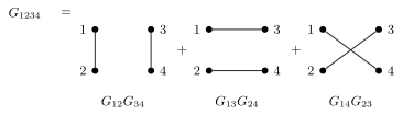
The real scalar four-point function is the sum of the three complete pairings of four labeled insertions. Each line represents one Feynman two-point function $G_{ij}$.

The four-point function is the first nontrivial example:

$$G_{1234} =G_{12}G_{34}+G_{13}G_{24}+G_{14}G_{23}.$$

The three terms are exactly the three ways of pairing four labeled points. The six-point function has

$$(6-1)!!=15$$

terms. In diagrammatic notation one rarely writes all fifteen products explicitly unless a particular labeling matters.

At this stage every labeled Wick pairing appears with coefficient $1$. Symmetry factors enter later for a different reason: when interaction vertices are integrated over and no longer labeled by fixed external positions, many algebraically distinct contractions can collapse to the same unlabeled topology. The symmetry factor of an interacting Feynman diagram counts that collapse. It is not an extra factor in the labeled Wick theorem itself.

Complex scalar fields and directed contractions

A complex scalar field has a global $U(1)$ symmetry. In the convention used throughout this course,

$$\phi\longrightarrow e^{-i\alpha}\phi, \qquad \phi^{\dagger}\longrightarrow e^{i\alpha}\phi^{\dagger}.$$

With $U(\alpha)=e^{i\alpha Q}$, this means

$$[Q,\phi]=-\phi, \qquad [Q,\phi^{\dagger}]=+\phi^{\dagger}.$$

These equations give the transformation charge of the field operators. They do not say that the particle annihilated by $\phi$ has charge $-1$: in the mode expansion, $a^{\dagger}$ creates a particle state of charge $+1$, while $b^{\dagger}$ creates an antiparticle state of charge $-1$. The field $\phi$ lowers the total charge by one because it annihilates the former or creates the latter.

The vacuum is neutral, so a vacuum expectation value must have total operator charge zero. Thus

$$\langle0|\mathcal T\phi(x_1)\cdots\phi(x_r) \phi^{\dagger}(y_1)\cdots\phi^{\dagger}(y_s)|0\rangle=0 \qquad\text{if }r\ne s.$$

In a free complex scalar theory the elementary nonzero contraction is

$$G(x|y)=\langle0|\mathcal T\phi(x)\phi^{\dagger}(y)|0\rangle.$$

The same-charge contractions vanish:

$$\langle0|\mathcal T\phi(x)\phi(y)|0\rangle=0, \qquad \langle0|\mathcal T\phi^{\dagger}(x)\phi^{\dagger}(y)|0\rangle=0.$$

This is why arrows are natural. Here a directed line records the ordered pairing $G(x|y)$ from its $\phi(x)$ endpoint to its $\phi^{\dagger}(y)$ endpoint. The arrow is a bookkeeping convention for the two different field types; once chosen, it must be used consistently.

For example,

$$\begin{aligned} &G(x_1,x_2|y_1,y_2) \\ &\quad\equiv \langle0|\mathcal T\phi(x_1)\phi(x_2) \phi^{\dagger}(y_1)\phi^{\dagger}(y_2)|0\rangle \\ &\quad= G(x_1|y_1)G(x_2|y_2) +G(x_1|y_2)G(x_2|y_1). \end{aligned}$$

The general formula is a sum over permutations:

$$\boxed{ G(x_1,\ldots,x_n|y_1,\ldots,y_n) = \sum_{\sigma\in S_n}\prod_{i=1}^n G(x_i|y_{\sigma(i)}). }$$

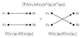
The complex scalar four-point function pairs each $\phi$ insertion with one $\phi^{\dagger}$ insertion. The two directed diagrams represent the two permutations of the $\phi^{\dagger}$ endpoint labels.

This is the complex-field analogue of the real-field pairing formula. The real scalar field sums over pair partitions of $2N$ objects. The complex scalar field sums over bijections from the $n$ insertions of $\phi$ to the $n$ insertions of $\phi^{\dagger}$.

The distinction becomes important as soon as interactions are present. A real $\phi^4$ vertex has four identical real lines. A complex interaction such as $(\phi^{\dagger}\phi)^2$ has two incoming charge lines and two outgoing charge lines. The diagram already knows the charge bookkeeping.

Connected and disconnected diagrams

The free real four-point function is not zero, but it is entirely disconnected:

$$G_{1234}=G_{12}G_{34}+G_{13}G_{24}+G_{14}G_{23}.$$

Each term is a product of two two-point functions. If we define the connected four-point function by subtracting all products of lower connected correlators, then for the free scalar field

$$G^{\mathrm{conn}}_{1234} =G_{1234}-G_{12}G_{34}-G_{13}G_{24}-G_{14}G_{23}=0.$$

This is the diagrammatic statement that free particles propagate but do not scatter. A two-point function is connected: one line connects its two insertions. A free four-point function is a sum of products of two independent propagations. It correlates four insertions only in the weak sense that the four insertions can be grouped into pairs.

It is helpful to separate three adjectives that often get blurred. Full correlators include everything, connected and disconnected. Connected correlators remove factorized products. Amputated correlators, introduced later, remove external propagators from connected correlators. Wick diagrams on this page are full free correlators unless explicitly labeled connected.

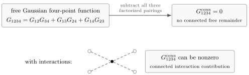
Free four-point Wick diagrams factorize into products of two propagators. After subtracting factorized pieces, the connected free four-point function vanishes. A genuine connected four-point graph first appears when an interaction vertex is inserted.

The same idea holds for all higher free correlators. The connected correlators of a Gaussian theory vanish except at two points:

$$G^{\mathrm{conn}}_n=0 \qquad\text{for }n\ne2$$

in a free theory with vanishing one-point function. This statement is sometimes called the vanishing of higher cumulants. It is the probabilistic heart of Wick theorem.

For complex fields, the connected part of

$$\langle0|\mathcal T\phi(x_1)\phi(x_2) \phi^{\dagger}(y_1)\phi^{\dagger}(y_2)|0\rangle$$

also vanishes in the free theory after subtracting

$$G(x_1|y_1)G(x_2|y_2)+G(x_1|y_2)G(x_2|y_1).$$

The arrows do not make the free theory interacting; they only record which pairings are allowed.

The wave equation as a diagrammatic rule

The free field obeys the operator equation

$$(\Box+m^2)\phi(x)=0.$$

Inside a time-ordered correlator this equation is modified by contact terms. The modification is not a failure of the field equation; it comes from differentiating the step functions hidden inside $\mathcal T$.

For a real scalar correlator,

$$G_n(x_1,\ldots,x_n) = \langle0|\mathcal T\phi(x_1)\cdots\phi(x_n)|0\rangle,$$

Wick theorem gives

$$\boxed{ (\Box_{x_1}+m^2)G_n(x_1,\ldots,x_n) =-i\sum_{j=2}^n\delta^{(4)}(x_1-x_j) G_{n-2}(x_2,\ldots,\widehat{x_j},\ldots,x_n). }$$

The hat means that the argument is omitted. Diagrammatically, acting with $\Box+m^2$ on the point $x_1$ collapses the line connecting $x_1$ to its partner. The collapse produces a delta function and removes both endpoints from the remaining diagram.

For a complex scalar field, the same idea is charge-selective. Acting on a $\phi(x_i)$ insertion can only collapse a line connecting it to a $\phi^{\dagger}(y_a)$ insertion:

$$\boxed{ (\Box_{x_i}+m^2)G(x_1,\ldots,x_n|y_1,\ldots,y_n) =-i\sum_{a=1}^n\delta^{(4)}(x_i-y_a) G(x_1,\ldots,\widehat{x_i},\ldots,x_n|y_1,\ldots,\widehat{y_a},\ldots,y_n). }$$

This is a compact way to see both the Green-function property and the charge-flow rule. A propagator is the inverse of the quadratic kinetic operator, but only between fields that can contract.

From Wick diagrams to perturbation theory

The free diagrams above contain only external insertions and contractions. Interactions enter through the Dyson expansion. This adds a new kind of point: an integration point coming from the action rather than an operator inserted by the observer.

That distinction matters. External points are labeled and fixed. Interaction vertices are integrated over spacetime. Symmetry factors arise because many labeled Wick contractions can collapse to the same unlabeled graph after the vertex coordinates are integrated.

The diagrams so far describe a free theory. Perturbation theory starts when the Dyson expansion inserts powers of the interaction Hamiltonian. Schematically, for an operator product $\mathcal O$ made from fields,

$$\langle\mathcal T\mathcal O\rangle = \frac{\langle0|\mathcal T\mathcal O\,\exp\left(-i\int dt\,V_I(t)\right)|0\rangle_0}{\langle0|\mathcal T\exp\left(-i\int dt\,V_I(t)\right)|0\rangle_0}.$$

The subscript $0$ means that the expectation value is evaluated in the free theory. Wick theorem is then applied to the larger product containing both the external fields in $\mathcal O$ and the fields inside the interaction $V_I$.

For instance, if an interaction contains four scalar fields at a time $t$, then a first-order term contains a free correlator of the form

$$-i\frac{\lambda}{4!}\int dt\,\langle0|\mathcal T\mathcal O\,\phi(t)^4|0\rangle_0.$$

The four fields at the same interaction point are represented by a vertex with four half-lines attached. Wick contractions then connect those half-lines either to external insertions or to other fields produced by interaction vertices. This is how the free Wick diagrams become the perturbative Feynman diagrams of an interacting theory.

This also explains why factorials must be treated carefully. The factor $1/4!$ in $\lambda\phi^4/4!$ compensates the number of ways to permute the four identical fields at a single labeled vertex. The factor $1/n!$ in the exponential expansion compensates the number of ways to permute $n$ identical interaction insertions. After these cancellations, a remaining symmetry factor may still appear if a graph has nontrivial automorphisms. The cleanest way to avoid mistakes is to begin with labeled Wick contractions and only then pass to unlabeled diagrams.

The denominator removes vacuum bubbles that are completely disconnected from the external insertions. This fact will become important once the path-integral generating functional is introduced: taking the logarithm of the generating functional selects connected diagrams, while further Legendre transforming selects one-particle-irreducible diagrams.

Gaussian moments behind the pictures

The bottom layer under Wick diagrams is ordinary Gaussian integration. In finite dimensions, let $K$ be a symmetric positive matrix and define

$$Z[J]=\int d^N\varphi\, \exp\left(-\frac12\varphi_iK_{ij}\varphi_j+J_i\varphi_i\right).$$

Completing the square gives

$$Z[J]=Z[0]\exp\left(\frac12J_iK^{-1}_{ij}J_j\right).$$

Moments are obtained by differentiating with respect to $J$:

$$\langle\varphi_{i_1}\cdots\varphi_{i_{2N}}\rangle = \left.\frac{1}{Z[0]} \frac{\partial}{\partial J_{i_1}}\cdots \frac{\partial}{\partial J_{i_{2N}}}Z[J]\right|_{J=0}.$$

Since the exponent is quadratic in $J$, differentiating produces only pairings:

$$\langle\varphi_{i_1}\cdots\varphi_{i_{2N}}\rangle = \sum_{\text{pairings }P}\prod_{(a,b)\in P}(K^{-1})_{i_a i_b}.$$

This is Wick theorem without time ordering, without operator language, and without relativity. The propagator is simply the inverse matrix $K^{-1}$.

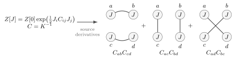
The finite-dimensional Gaussian generating function already contains Wick theorem. Differentiating $Z[J]$ four times produces the three pairings of four source labels.

For a convergent complex Gaussian, integrate over $z\in\mathbb C^N$ with $\bar z=z^*$ on the integration contour, and take $K$ to be Hermitian positive definite. Write

$$Z[\eta,\bar\eta] =\int_{\mathbb C^N}d^{2N}z\, \exp\left(-\bar z_iK_{ij}z_j+\bar\eta_i z_i+\bar z_i\eta_i\right).$$

Here $d^{2N}z=\prod_i d\operatorname{Re}z_i\,d\operatorname{Im}z_i$. The source variables $\eta$ and $\bar\eta$ may be treated as algebraically independent when taking derivatives; this does not turn $z$ and $\bar z$ into independent complex integration coordinates.

Then

$$Z[\eta,\bar\eta]=Z[0,0] \exp\left(\bar\eta_iK^{-1}_{ij}\eta_j\right),$$

so nonzero moments pair $z$ only with $\bar z$:

$$\langle z_{i_1}\cdots z_{i_n}\bar z_{j_1}\cdots\bar z_{j_n}\rangle = \sum_{\sigma\in S_n}\prod_{a=1}^n (K^{-1})_{i_a j_{\sigma(a)}}.$$

This is exactly the directed contraction rule for a complex scalar field. The next page will turn this finite-dimensional Gaussian identity into the path integral for quantum mechanics and fields.

Summary

A safe way to draw a free Wick diagram is: list the external insertions, draw every allowed complete pairing exactly once, translate each line into a propagator, and then add the resulting products. For complex fields, impose charge flow before drawing any line.

A Wick diagram is an algebraic term written as a picture. For a real scalar field, every complete pairing of insertions contributes one product of propagators. The four-point function has three pairings, the six-point function has fifteen, and in general the $2N$-point function has $(2N-1)!!$ terms.

For a complex scalar field, the global $U(1)$ charge eliminates same-charge contractions. A correlator with $n$ fields $\phi$ and $n$ fields $\phi^{\dagger}$ is a sum over $n!$ directed pairings,

$$G(x_1,\ldots,x_n|y_1,\ldots,y_n) = \sum_{\sigma\in S_n}\prod_{i=1}^nG(x_i|y_{\sigma(i)}),$$

while correlators with unequal numbers of $\phi$ and $\phi^{\dagger}$ vanish.

The connected part of every free correlator beyond the two-point function vanishes. This is the diagrammatic meaning of “free”: the field can propagate between insertions, but it cannot produce genuine multi-point scattering. Interaction vertices are precisely what will create connected higher-point diagrams.

Finally, the same pairing rules follow from finite-dimensional Gaussian integrals. The propagator is the inverse of the quadratic operator, and diagrams are a disciplined notation for differentiating a Gaussian generating function.

Common pitfalls

A Wick line is not literally the path of a particle through spacetime. It is a two-point Green function. Thinking of it as a classical trajectory often leads to wrong intuition, especially in loop diagrams.

Do not add symmetry factors to labeled free correlators. In

$$G_{1234}=G_{12}G_{34}+G_{13}G_{24}+G_{14}G_{23},$$

each term has coefficient $1$. Symmetry factors appear later when many labeled Wick contractions correspond to the same unlabeled interacting diagram.

For complex fields, do not draw contractions between two $\phi$ insertions or two $\phi^{\dagger}$ insertions in the charge-conserving free vacuum. Such lines violate the $U(1)$ selection rule.

Disconnected does not mean unimportant. Disconnected pieces are part of ordinary correlation functions. They disappear only after forming connected correlators or after taking the logarithm of an appropriate generating functional.

The free equation of motion holds inside correlators only away from contact points. At coincident insertions, time ordering produces delta functions.

Exercises

Exercise 1: Real scalar six-point diagrams

Write the real scalar six-point function in the form obtained by first pairing the insertion $1$ with one of the other insertions.

Solution

Pair insertion $1$ with one of $2,3,4,5,6$. For each choice, the remaining four labels have three pairings. Therefore

$$\begin{aligned} G_{123456}={}& G_{12}(G_{34}G_{56}+G_{35}G_{46}+G_{36}G_{45})\\ &+G_{13}(G_{24}G_{56}+G_{25}G_{46}+G_{26}G_{45})\\ &+G_{14}(G_{23}G_{56}+G_{25}G_{36}+G_{26}G_{35})\\ &+G_{15}(G_{23}G_{46}+G_{24}G_{36}+G_{26}G_{34})\\ &+G_{16}(G_{23}G_{45}+G_{24}G_{35}+G_{25}G_{34}). \end{aligned}$$

There are $5\times3=15$ terms, as required by $(6-1)!!=15$.

Exercise 2: Directed complex scalar contractions

Let $\phi$ be a free complex scalar field. Compute

$$\langle0|\mathcal T\phi(x_1)\phi(x_2)\phi(x_3) \phi^{\dagger}(y_1)\phi^{\dagger}(y_2)\phi^{\dagger}(y_3)|0\rangle.$$

Solution

Only $\phi$–$\phi^{\dagger}$ contractions are nonzero. Therefore the result is a sum over all permutations of $y_1,y_2,y_3$:

$$\begin{aligned} G(x_1,x_2,x_3|y_1,y_2,y_3) ={}&G(x_1|y_1)G(x_2|y_2)G(x_3|y_3)\\ &+G(x_1|y_1)G(x_2|y_3)G(x_3|y_2)\\ &+G(x_1|y_2)G(x_2|y_1)G(x_3|y_3)\\ &+G(x_1|y_2)G(x_2|y_3)G(x_3|y_1)\\ &+G(x_1|y_3)G(x_2|y_1)G(x_3|y_2)\\ &+G(x_1|y_3)G(x_2|y_2)G(x_3|y_1). \end{aligned}$$

Equivalently,

$$G(x_1,x_2,x_3|y_1,y_2,y_3) =\sum_{\sigma\in S_3}\prod_{i=1}^3G(x_i|y_{\sigma(i)}).$$

There are $3!=6$ directed pairings.

Exercise 3: Connected four-point function

For a free real scalar field with vanishing one-point function, show that the connected four-point function vanishes.

Solution

The full four-point function is

$$G_{1234}=G_{12}G_{34}+G_{13}G_{24}+G_{14}G_{23}.$$

For a theory with $\langle\phi\rangle=0$, the connected four-point function is defined by subtracting the products of connected two-point functions:

$$G^{\mathrm{conn}}_{1234} =G_{1234}-G_{12}G_{34}-G_{13}G_{24}-G_{14}G_{23}.$$

Substituting the Wick expansion gives

$$G^{\mathrm{conn}}_{1234}=0.$$

This is the simplest example of the general statement that a Gaussian theory has no connected correlators beyond two points.

Exercise 4: Gaussian four-point moment

Starting from the finite-dimensional Gaussian generating function

$$Z[J]=Z[0]\exp\left(\frac12J_iK^{-1}_{ij}J_j\right),$$

compute $\langle\varphi_a\varphi_b\varphi_c\varphi_d\rangle$.

Solution

By definition,

$$\langle\varphi_a\varphi_b\varphi_c\varphi_d\rangle =\left.\frac{1}{Z[0]} \frac{\partial}{\partial J_a} \frac{\partial}{\partial J_b} \frac{\partial}{\partial J_c} \frac{\partial}{\partial J_d}Z[J]\right|_{J=0}.$$

Only terms quadratic squared in the exponential contribute. Since

$$\exp\left(\frac12J_iK^{-1}_{ij}J_j\right) =1+\frac12J_iK^{-1}_{ij}J_j +\frac18J_iK^{-1}_{ij}J_jJ_kK^{-1}_{k\ell}J_{\ell}+\cdots,$$

four derivatives pick out the three pairings of the four source labels. Thus

$$\boxed{ \langle\varphi_a\varphi_b\varphi_c\varphi_d\rangle =(K^{-1})_{ab}(K^{-1})_{cd} +(K^{-1})_{ac}(K^{-1})_{bd} +(K^{-1})_{ad}(K^{-1})_{bc}. }$$

This is precisely the four-point Wick formula with $K^{-1}$ playing the role of the propagator.

Exercise 5: Complex Gaussian pairings

For the complex Gaussian

$$Z[\eta,\bar\eta]=Z[0,0]\exp(\bar\eta_iK^{-1}_{ij}\eta_j),$$

show that

$$\langle z_a z_b\bar z_c\bar z_d\rangle =(K^{-1})_{ac}(K^{-1})_{bd}+(K^{-1})_{ad}(K^{-1})_{bc}.$$

Solution

The expectation value is obtained by differentiating once with respect to the source for each variable. With the conventions in the text,

$$\langle z_a z_b\bar z_c\bar z_d\rangle =\left. \frac{1}{Z[0,0]} \frac{\partial}{\partial\bar\eta_a} \frac{\partial}{\partial\bar\eta_b} \frac{\partial}{\partial\eta_c} \frac{\partial}{\partial\eta_d} Z[\eta,\bar\eta] \right|_{\eta=\bar\eta=0}.$$

The exponent contains only mixed products $\bar\eta_iK^{-1}_{ij}\eta_j$. Therefore every $z$ source must be paired with a $\bar z$ source. The two possible pairings are

$$a\leftrightarrow c, \quad b\leftrightarrow d,$$

and

$$a\leftrightarrow d, \quad b\leftrightarrow c.$$

Thus

$$\langle z_a z_b\bar z_c\bar z_d\rangle =(K^{-1})_{ac}(K^{-1})_{bd}+(K^{-1})_{ad}(K^{-1})_{bc}.$$

This is the finite-dimensional version of the complex scalar four-point formula.

References and further reading

• Sidney Coleman, Lectures of Sidney Coleman on Quantum Field Theory, Chapter 8, for Wick diagrams, connected and disconnected diagrams, and the organization of perturbation theory.
• Mark Srednicki, Quantum Field Theory, Sections 8–10, for the path-integral derivation of free-field correlators and the transition to Feynman rules.
• Steven Weinberg, The Quantum Theory of Fields, Volume I, Sections 6.1–6.2, for Wick pairings, coordinate-space Feynman rules, and propagators.
• A. Zee, Quantum Field Theory in a Nutshell, Appendix A and Chapter I.7, for Gaussian integration and the physical meaning of diagrammatic expansion.