Effective Actions in Background Fields

The previous page introduced functional determinants and proper time. We now put that technology to work in the cleanest possible laboratory: a charged quantum field moving in a fixed electromagnetic background. The background is not dynamical at first. It is a probe. By integrating out the charged matter, we ask what local and nonlocal terms are induced in the effective action for the background field.

The payoff is large. A constant magnetic field diagonalizes the one-loop problem into Landau levels, so the determinant can be computed without drawing a single momentum-space diagram. The same answer knows about vacuum polarization, charge renormalization, magnetic susceptibility, and the finite nonlinear photon interactions that become the Euler–Heisenberg effective action. It also reveals a physical distinction that will be crucial for Yang–Mills theory: orbital motion tends to screen, while spin magnetic moments can produce the opposite sign.

Required background. Proper Time, Determinants, and Thermal Traces supplies the determinant signs, heat-kernel normalization, and the open-to-closed worldline construction. Running Charge, Screening, and Antiscreening fixes the interpretation of positive matter contributions to $1/e^2$. The signs below refer first to the coefficient of $F^2$ in the effective action, $\Gamma[A]\supset(4e^2)^{-1}\int F^2$, not directly to the beta function. A positive logarithmic contribution from modes between $m$ and $\Lambda$ raises $1/e^2$; differentiating with respect to the renormalization scale then gives the familiar positive QED beta function.

Background fields and one-loop determinants

Determinant and heat-kernel normalization

We use the Euclidean rescaled gauge-field normalization from the previous pages,

$$\Gamma[A]\supset {1\over4}\int d^4x\,{1\over e^2}F_{\mu\nu}F_{\mu\nu},$$

and charged matter has unit charge,

$$D_\mu=\partial_\mu-iA_\mu, \qquad [D_\mu,D_\nu]=-iF_{\mu\nu}.$$

Take smooth real Euclidean backgrounds and $m>0$. The scalar and squared Dirac operators use self-adjoint, covariant realizations; in a finite-volume problem the heat traces must be trace class. Every constant-field trace divided by $V_4$ below means the infinite-volume bulk density, with continuous momenta in the two free directions. It excludes hard-wall edge corrections and finite-temperature Matsubara sums. The preceding lesson states the zero-mode and boundary qualifications. For a pure magnetic background choose $B>0$ without loss of generality,

$$F_{12}=B, \qquad F_{\mu\nu}F_{\mu\nu}=2B^2.$$

A complex scalar contributes

$$\Gamma_s^{(1)}[A]=\operatorname{Tr}\log(-D^2+m^2),$$

while a Dirac fermion contributes

$$\Gamma_f^{(1)}[A]=- \operatorname{Tr}\log(\gamma_\mu D_\mu+m).$$

The signs come from ordinary Gaussian integration: bosonic determinants sit in the denominator of the path integral, Grassmann determinants sit in the numerator.

Let $\chi$ denote a charged quantum field and let $A_\mu$ be a fixed external field. The effective action for $A_\mu$ is defined by

$$e^{-\Gamma[A]} = \int \mathcal D\chi\,e^{-S_E[\chi,A]}.$$

If $\chi$ is a complex scalar with

$$S_E[\phi,A] = \int d^4x\,\phi^*(-D^2+m^2)\phi,$$

then the matter integral is Gaussian and gives

$$e^{-\Gamma_s^{(1)}[A]} \propto \left[\operatorname{Det}(-D^2+m^2)\right]^{-1}.$$

Therefore

$$\Gamma_s^{(1)}[A] = \operatorname{Tr}\log(-D^2+m^2).$$

For a Dirac fermion,

$$S_E[\psi,A] = \int d^4x\,\overline\psi(\gamma_\mu D_\mu+m)\psi,$$

and Grassmann integration gives

$$e^{-\Gamma_f^{(1)}[A]} \propto \operatorname{Det}(\gamma_\mu D_\mu+m),$$

so

$$\Gamma_f^{(1)}[A] =-\operatorname{Tr}\log(\gamma_\mu D_\mu+m).$$

The trace includes spacetime, spinor indices when present, and any internal indices. The determinant is a compact way to sum all one-loop diagrams with external $A_\mu$ insertions. This is also why background fields are so efficient pedagogically: one calculation of a spectral trace contains the two-point vacuum polarization, four-photon scattering, and all higher one-loop background vertices.

This defines integrating out a heavy charged field, as in Schwartz 2014, § 33.3, pp. 711–712. Slowly varying backgrounds permit a local derivative expansion when their variation scales are small compared with $m$. Truncating also in powers of field strength requires the separate weak-field condition $|F|/m^2\ll1$. A constant field can have arbitrary strength despite having no gradients. At external energies comparable with $m$, the determinant has nonlocal, threshold-dependent terms and needs the appropriate continuation.

To see the diagrammatic expansion explicitly, start with finite-regulator algebra and write

$$L_A=L_0+V[A], \qquad G_0=L_0^{-1}.$$

Then

$$\operatorname{Tr}\log L_A = \operatorname{Tr}\log L_0+\operatorname{Tr}\log(1+G_0V),$$

and therefore

$$\operatorname{Tr}\log L_A = \operatorname{Tr}\log L_0 +\operatorname{Tr}(G_0V) -{1\over2}\operatorname{Tr}(G_0VG_0V) +{1\over3}\operatorname{Tr}(G_0VG_0VG_0V)-\cdots.$$

Powers of $V$ count vertices, not photons. For the scalar Laplacian,

$$V=V_1+V_2,\qquad V_1=i(\partial\!\cdot\! A)+2iA\!\cdot\!\partial,\qquad V_2=A^2.$$

Set $X=G_0V_1$ and $Y=G_0V_2$. Replacing $A\mapsto tA$ gives $G_0V=tX+t^2Y$. Collecting powers of $t$ yields

$$\begin{aligned} \left(\Delta\Gamma_s^{(1)}\right)_{A^2} &=\operatorname{Tr}Y-\frac12\operatorname{Tr}X^2,\\ \left(\Delta\Gamma_s^{(1)}\right)_{A^4} &=-\frac12\operatorname{Tr}Y^2 +\operatorname{Tr}(X^2Y)-\frac14\operatorname{Tr}X^4. \end{aligned}$$

The mixed term comes from $\operatorname{Tr}(X^2Y+XYX+YX^2)/3$ and cyclicity. Thus scalar vacuum polarization contains a seagull and a bubble; four-photon scattering contains two seagulls, a mixed triangle and a box. Omitting contact vertices spoils the gauge response. Current Sources and Generating Functionals derives the same scalar contact from source differentiation.

The unsquared Dirac operator is linear in $A$, so its expansion has only one-photon vertices and a fermion-loop sign. Its squared Laplace-type representation contains $A^2$ again, as well as the linear spin coupling, and has the overall $-1/2$ factor. These are alternative organizations of the same parity-even answer. The following scalar diagram groups terms by photon number; every group must receive one consistent regulator.

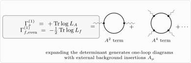
The scalar determinant must be collected by powers of $A$, with $X=G_0V_1$ and $Y=G_0V_2$. A filled vertex with two photon legs represents $V_2$. The displayed traces give the complete quadratic and quartic groups in finite-regulator algebra; the pictures indicate topology, not additional symmetry factors or momenta. The first-order Dirac organization differs as explained above.

A useful identity for variations is

$$\delta\operatorname{Tr}\log L = \operatorname{Tr}(L^{-1}\delta L).$$

This is ordinary finite-dimensional logarithm algebra. A proper-time cutoff changes its form. For a positive self-adjoint $L$, define

$$F_\epsilon(L)=-\int_\epsilon^\infty\frac{ds}{s}\, \operatorname{Tr}e^{-sL}.$$

Assume a common operator domain and enough trace bounds to differentiate under this integral; finite matrices provide a direct check. Duhamel’s formula and cyclicity give

$$\begin{aligned} \delta\operatorname{Tr}e^{-sL} &=-\int_0^sdu\,\operatorname{Tr} \left(e^{-(s-u)L}\delta L\,e^{-uL}\right)\\ &=-s\operatorname{Tr}(e^{-sL}\delta L),\\ \delta F_\epsilon(L) &=\operatorname{Tr}\left(e^{-\epsilon L}L^{-1}\delta L\right). \end{aligned}$$

The filter $e^{-\epsilon L}$ is essential at fixed cutoff. For example, for $L=\lambda>0$, direct differentiation gives $e^{-\epsilon\lambda}/\lambda$ instead of $1/\lambda$. Taking $\epsilon\to0$ inside a field-theory trace without counterterms is not justified. Even the quadratic background coefficient has the cutoff-dependent form

$$\begin{aligned} \left(F_\epsilon(L_A)-F_\epsilon(L_0)\right)_{A^2} =\int_\epsilon^\infty ds\,\Bigl[&\operatorname{Tr}(V_2e^{-sL_0})\\ &-\frac{s}{2}\int_0^1du\, \operatorname{Tr}\left(V_1e^{-suL_0}V_1e^{-s(1-u)L_0}\right)\Bigr]. \end{aligned}$$

At $\epsilon=0$ in finite dimensions, the two integrals reduce to $\operatorname{Tr}(G_0V_2)$ and $\operatorname{Tr}(G_0V_1G_0V_1)/2$. The cutoff formula keeps the same two topologies while regulating them together. Local counterterms and their variations must then be included in a renormalized response.

In a regulated Euclidean functional integral define the source current by $J_\mu(x)\equiv\delta S_E/\delta A_\mu(x)$. Differentiating the same regulated $\Gamma[A]=-\log Z[A]$ gives

$${\delta\Gamma[A]\over\delta A_\mu(x)}=\langle J_\mu(x)\rangle_A.$$

The determinant prescription and the current insertion must use the same regulator. Euclidean derivatives determine Euclidean response kernels; after continuation, an in-out functional gives time-ordered amplitudes. A retarded response is a different real-time prescription.

The worldline representation from the previous page makes the same response geometric. For a complex scalar with $D_\mu=\partial_\mu-iA_\mu$,

$$\boxed{ \Gamma_s^{(1)}[A]-\Gamma_s^{(1)}[0] =-\int_\epsilon^\infty {ds\over s}\,e^{-m^2s} \int_{x(s)=x(0)}\!\mathcal D x\, e^{-\int_0^s d\tau\,\dot x^2/4} \left(e^{+i\oint A_\mu dx^\mu}-1\right). }$$

The subtraction removes the field-independent closed loops. Reversing a loop’s orientation complex-conjugates its Wilson phase, so odd powers of an Abelian background cancel in the unoriented loop average. The first local response is therefore quadratic in $F_{\mu\nu}$, exactly as required by gauge invariance and as found from vacuum polarization.

Proper time in a magnetic field

The proper-time representation turns the determinant into a spectral trace. For a complex scalar,

$$\Gamma_s^{(1)}[A] = -\int_\epsilon^\infty {ds\over s}\, \operatorname{Tr}\,e^{-s(-D^2+m^2)} +\text{counterterms},$$

where $\epsilon\sim \Lambda^{-2}$ is a gauge-covariant ultraviolet cutoff. In the proper-time formulas below, $\Gamma^{(1)}$ denotes this cutoff matter contribution before counterterms. Subtracting the field-independent vacuum term gives

$$\Gamma_s^{(1)}[A]-\Gamma_s^{(1)}[0] = -\int_\epsilon^\infty {ds\over s}\,e^{-m^2s} \operatorname{Tr}\left(e^{sD^2}-e^{s\partial^2}\right).$$

Now choose a constant magnetic field in the $x^3$ direction,

$$F_{12}=B,$$

and take the gauge

$$A_2=Bx_1, \qquad A_1=A_3=A_4=0.$$

The transverse operator is

$$-D_1^2-D_2^2 = -\partial_1^2-(\partial_2-iBx_1)^2.$$

At fixed momentum $p_2$, this is a harmonic oscillator in $x_1$ with frequency $B$. Its eigenvalues are

$$(2n+1)B, \qquad n=0,1,2,\ldots.$$

The two remaining Euclidean directions are free, so the full scalar spectrum is

$$\lambda_{n,p_3,p_4}=p_3^2+p_4^2+(2n+1)B.$$

The degeneracy per unit area in the $x^1x^2$ plane is

$${B\over2\pi}.$$

Therefore the scalar heat kernel per four-volume is

$${1\over V_4}\operatorname{Tr}e^{-s(-D^2)} = {B\over2\pi}\sum_{n=0}^\infty e^{-s(2n+1)B} \int {d^2p_\parallel\over(2\pi)^2}e^{-sp_\parallel^2},$$

where $p_\parallel=(p_3,p_4)$. Since

$$\int {d^2p_\parallel\over(2\pi)^2}e^{-sp_\parallel^2}={1\over4\pi s}$$

and

$$\sum_{n=0}^\infty e^{-s(2n+1)B} ={1\over2\sinh Bs},$$

we obtain

$$\boxed{ {1\over V_4}\operatorname{Tr}e^{-s(-D^2)} ={1\over(4\pi s)^2}{Bs\over\sinh Bs}. }$$

The figure compares the scalar ladder with the two spin-shifted ladders derived below. The coincident positive spinor levels, rather than an alternating sequence, produce the $\coth(Bs)$ heat trace.

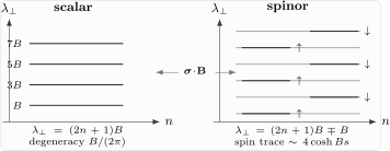
The exact transverse scalar levels are $(2n+1)B$ for $B>0$. The squared Dirac operator has ladders $2nB$ and $2(n+1)B$, each with internal multiplicity two: all positive levels coincide, and only one spin sector has a transverse zero level. Both carry orbital density $B/(2\pi)$ per unit area. Adding $p_\parallel^2+m^2$ makes the full eigenvalue positive for $m>0$. The finite subset of levels is schematic; their spacing and coincidences are exact.

The magnetic field has converted the problem into a product of two familiar ingredients: free heat flow in the directions parallel to the field and harmonic-oscillator heat flow in the transverse plane.

Scalar QED: orbital response and the local F² term

The scalar effective action in a constant magnetic field is

$${\Gamma_s^{(1)}[B]-\Gamma_s^{(1)}[0]\over V_4} = -\int_\epsilon^\infty {ds\over s}\,e^{-m^2s} {1\over(4\pi s)^2} \left({Bs\over\sinh Bs}-1\right).$$

The small-$s$ region controls the ultraviolet divergence. For $x=Bs$,

$${x\over\sinh x}=1-{x^2\over6}+{7x^4\over360}+O(x^6).$$

Thus the first field-dependent term in the effective action is

$${\Gamma_s^{(1)}[B]\over V_4} \supset {B^2\over6(4\pi)^2} \int_\epsilon^\infty {ds\over s}\,e^{-m^2s}.$$

The logarithmic part is

$$\int_\epsilon^\infty {ds\over s}\,e^{-m^2s} = \log {1\over m^2\epsilon}+\text{finite} = \log {\Lambda^2\over m^2}+\text{finite}.$$

Therefore

$$\Gamma_s^{(1)}[B] \supset {V_4B^2\over96\pi^2}\log {\Lambda^2\over m^2}.$$

Because $F_{\mu\nu}F_{\mu\nu}=2B^2$, this is

$$\Gamma_s^{(1)}[A] \supset {1\over192\pi^2}\log {\Lambda^2\over m^2} \int d^4x\,F_{\mu\nu}F_{\mu\nu}.$$

Matching to

$${1\over4}\int d^4x\,{1\over e^2}F_{\mu\nu}F_{\mu\nu}$$

gives the scalar contribution. The factor of $1/4$ in the Maxwell term is easy to miss: the coefficient of $\int F^2$ in $\Gamma$ must be multiplied by $4$ to obtain the shift of $1/e^2$.

$$\boxed{ \Delta\left({1\over e^2}\right)_s = {1\over48\pi^2}\log {\Lambda^2\over m^2} = {1\over16\pi^2}{1\over3}\log {\Lambda^2\over m^2}. }$$

This is the same coefficient found from the momentum-space vacuum polarization, now derived from a constant-background heat kernel.

The factor $x/\sinh x$ is less than one for real nonzero $x$. In the thermodynamic language of a charged particle, the orbital motion in a magnetic field reduces the density of low-lying states compared with the naive classical phase-space result. This is the origin of the word diamagnetic in this discussion. In field theory the observable statement is the induced local $F^2$ term; the separation into “magnetic susceptibility” language is an interpretation of the same coefficient.

Spinor QED: spin trace and paramagnetism

For a Dirac fermion, it is useful to square the Dirac operator. Up to an $A$-independent normalization and a choice of determinant branch, the parity-even part may be written as

$$\Gamma_f^{(1)}[A] =-{1\over2}\operatorname{Tr}\log\left[-(\gamma_\mu D_\mu)^2+m^2\right].$$

This rewriting is a calculational device for the even-in-$F$ part of the determinant. It is not a harmless replacement when one studies phases, spectral asymmetry, or anomalies.

Using

$$(\gamma_\mu D_\mu)^2 =D^2-{i\over4}[\gamma_\mu,\gamma_\nu]F_{\mu\nu},$$

the Laplace-type operator is

$$-(\gamma_\mu D_\mu)^2+m^2 = -D^2+m^2+{i\over4}[\gamma_\mu,\gamma_\nu]F_{\mu\nu}.$$

Hermitian Euclidean $\gamma_\mu$ and an anti-Hermitian $\gamma_\mu D_\mu$ on the stated domain imply $-(\gamma_\mu D_\mu)^2\geq0$, so adding $m^2>0$ makes the full operator positive. The last term is the spin magnetic moment. For $F_{12}=B>0$, it has eigenvalues $+B$ and $-B$, each twice degenerate in four-component Dirac notation. The transverse ladders are therefore $2nB$ and $2(n+1)B$: every positive level occurs in both sectors, while the transverse zero level occurs in one sector. This agrees with Dunne 2004, Eq. (1.44), PDF p. 16, with $eB$ absorbed into our $B$. The zero transverse level is not a zero eigenvalue of the full massive operator.

Summing the two ladders with their internal multiplicity two gives $2(1+2\sum_{n\geq1}e^{-2nBs})=2\coth(Bs)$. Multiplication by the Landau density $B/(2\pi)$ and the parallel Gaussian $1/(4\pi s)$ gives the spinor heat kernel per four-volume:

$$\boxed{ {1\over V_4}\operatorname{Tr}e^{-s[-(\gamma_\mu D_\mu)^2]} ={4\over(4\pi s)^2}\,Bs\coth Bs. }$$

Equivalently,

$$4Bs\coth Bs =4{Bs\over\sinh Bs}\cosh Bs.$$

The one-loop spinor effective action is therefore

$${\Gamma_f^{(1)}[B]-\Gamma_f^{(1)}[0]\over V_4} = {1\over2}\int_\epsilon^\infty {ds\over s}\,e^{-m^2s} {4\over(4\pi s)^2}\left(Bs\coth Bs-1\right).$$

For small $x$,

$$x\coth x=1+{x^2\over3}-{x^4\over45}+O(x^6).$$

Thus

$${\Gamma_f^{(1)}[B]\over V_4} \supset {2B^2\over3(4\pi)^2} \int_\epsilon^\infty {ds\over s}\,e^{-m^2s},$$

and hence

$$\Gamma_f^{(1)}[A] \supset {1\over48\pi^2}\log {\Lambda^2\over m^2} \int d^4x\,F_{\mu\nu}F_{\mu\nu}.$$

Matching again to the Maxwell term gives

$$\boxed{ \Delta\left({1\over e^2}\right)_f = {1\over12\pi^2}\log {\Lambda^2\over m^2} = {1\over16\pi^2}{4\over3}\log {\Lambda^2\over m^2}. }$$

The factor $4/3$ has a useful physical decomposition. Write

$$4{x\over\sinh x}\cosh x = 4\left(1-{x^2\over6}+\cdots\right) \left(1+{x^2\over2}+\cdots\right).$$

The coefficient of $x^2$ is

$$4\left(-{1\over6}+{1\over2}\right) =-{2\over3}+2={4\over3}.$$

The $-2/3$ term is the orbital contribution of four fermion components. The $+2$ term is the spin contribution. The spin term dominates. This is the cleanest elementary version of the paramagnetic mechanism that later reappears for spin-one gauge bosons.

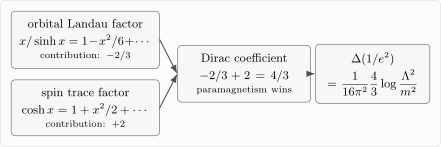
The orbital Landau-level factor $x/\sinh x$ begins with a negative $x^2$ correction, while the spin factor $\cosh x$ begins with a positive one. For a Dirac fermion the spin contribution is larger, giving the total coefficient $4/3$.

Renormalized constant-field actions

The proper-time integrals above still display the vacuum-energy and charge-renormalization terms. Once the zero-field vacuum term and the $B^2$ term have been fixed by renormalization conditions, the remaining constant-field action is finite. For one complex scalar,

$$\boxed{ {\Gamma_{s,\mathrm{ren}}^{(1)}(B)\over V_4} =-{1\over16\pi^2}\int_0^\infty {ds\over s^3}\,e^{-m^2s} \left[{Bs\over\sinh Bs}-1+{(Bs)^2\over6}\right]. }$$

For one Dirac fermion, the parity-even part is

$$\boxed{ {\Gamma_{f,\mathrm{ren}}^{(1)}(B)\over V_4} ={1\over8\pi^2}\int_0^\infty {ds\over s^3}\,e^{-m^2s} \left[Bs\coth Bs-1-{(Bs)^2\over3}\right]. }$$

The subtraction signs are fixed by the small-$s$ expansions, not chosen by magnetic intuition. They remove the $B^0$ and $B^2$ terms already assigned to the cosmological constant and the renormalized Maxwell coupling. The first surviving terms are finite:

$${\Gamma_{s,\mathrm{ren}}^{(1)}(B)\over V_4} =-{7B^4\over5760\pi^2m^4}+O(B^6/m^8),$$

and

$${\Gamma_{f,\mathrm{ren}}^{(1)}(B)\over V_4} =-{B^4\over360\pi^2m^4}+O(B^6/m^8).$$

These Euclidean signs are consistent with the familiar positive nonlinear magnetic terms in the Minkowski Lagrangian because a static effective action and a Minkowski Lagrangian differ by the Wick-rotation sign. More importantly, the coefficients are regulator-independent low-energy matching data once the $F^2$ term has been renormalized.

Gauge-covariant cutoffs

A sharp cutoff $|p|<\Lambda$ is natural in ordinary momentum integrals, but it is not gauge invariant in a general background field. Momentum is not a gauge-covariant label once $A_\mu(x)$ is present. A condition such as

$$|p-A(x)|<\Lambda$$

is not a clean gauge-invariant regulator either; it depends on a local gauge choice and does not define a spectral cutoff on a gauge-covariant operator.

The proper-time cutoff is better because it regulates the spectrum of a covariant operator:

$$\operatorname{Tr}\log L \longrightarrow -\int_{1/\Lambda^2}^\infty {ds\over s}\,\operatorname{Tr}e^{-sL}.$$

If $L$ transforms by conjugation under a gauge transformation,

$$L\mapsto g^{-1}Lg,$$

then

$$\operatorname{Tr}e^{-sL}$$

is gauge invariant. This is why the heat-kernel expansion organizes ultraviolet divergences directly into gauge-invariant local operators,

$$\int d^4x\,1, \qquad \int d^4x\,F_{\mu\nu}F_{\mu\nu}, \qquad \int d^4x\,(D_\rho F_{\mu\nu})(D_\rho F_{\mu\nu}), \qquad\ldots.$$

The first term is vacuum energy. The second renormalizes the gauge coupling. The later terms are higher-derivative effective interactions suppressed by powers of the mass or cutoff.

A related point is that the $F^2$ term extracted above is local. Its finite part depends on the renormalization convention. By contrast, after the $F^2$ coefficient is fixed at a reference scale, the higher-order low-energy terms such as $F^4/m^4$ are genuine predictions of the one-loop theory.

Preview: background-field gauge

The same background-field logic applies to Yang–Mills theory, but now the field being integrated out is partly the gauge field itself. The Abelian sections above use a Hermitian field $A_\mu$ in $D_\mu=\partial_\mu-iA_\mu$. For the non-Abelian preview, it is convenient to absorb the factor $-i$ into an anti-Hermitian Lie-algebra-valued connection,

$$\mathcal A_\mu\equiv -iA_\mu^aT^a, \qquad \mathcal D_\mu=\partial_\mu+\mathcal A_\mu.$$

This is a notation change, not a change of physical convention. Split

$$\mathcal A_\mu=\overline{\mathcal A}_\mu+a_\mu,$$

where $\overline{\mathcal A}_\mu$ is the background and $a_\mu$ is the quantum fluctuation. A background gauge transformation acts as

$$\overline{\mathcal A}_\mu \mapsto g^{-1}\overline{\mathcal A}_\mu g+g^{-1}\partial_\mu g, \qquad a_\mu\mapsto g^{-1}a_\mu g.$$

Thus the fluctuation transforms homogeneously, like matter in the adjoint representation. The background covariant derivative

$$\overline{\mathcal D}_\mu a_\nu = \partial_\mu a_\nu+[\overline{\mathcal A}_\mu,a_\nu]$$

also transforms homogeneously. This makes the gauge-fixing condition

$$\overline{\mathcal D}_\mu a_\mu=0$$

natural: it fixes the quantum gauge redundancy while preserving manifest gauge invariance with respect to the background.

In background Feynman gauge, the quadratic operator for gauge fluctuations has the schematic form

$$\mathcal L_{\mu\nu}^{\rm vec} = -\overline{\mathcal D}^{2}\delta_{\mu\nu} -2\operatorname{ad}(\overline{\mathcal F}_{\mu\nu}),$$

where

$$\operatorname{ad}(\overline{\mathcal F}_{\mu\nu})a_\nu =[\overline{\mathcal F}_{\mu\nu},a_\nu].$$

The associated ghosts contribute the scalar adjoint operator

$$\mathcal L_{\rm gh}=-\overline{\mathcal D}^{2}.$$

The term proportional to $\overline{\mathcal F}_{\mu\nu}$ is the spin-one magnetic-moment coupling of the vector fluctuation. It is the non-Abelian analog of the spin term in the squared Dirac operator, but with a larger spin response. After subtracting unphysical ghost modes, this paramagnetic spin-one term dominates the orbital screening part. That dominance is the physical seed of Yang–Mills antiscreening.

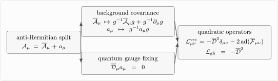
In the background-field method, $\mathcal A_\mu=\overline{\mathcal A}_\mu+a_\mu$. The background transforms as a connection, while the fluctuation transforms homogeneously. The quadratic vector operator contains a spin-one coupling to $\overline{\mathcal F}_{\mu\nu}$, and ghosts remove the unphysical scalar-like components.

This local ultraviolet calculation does not establish positivity of the full vector fluctuation operator. Some non-Abelian magnetic backgrounds have unstable modes, so a global determinant can require additional contour and infrared analysis even while its local $F^2$ divergence is well defined; Dunne 2004, § 3, Eq. (3.9), PDF p. 39 discusses this distinction. The next page turns the ultraviolet calculation into the beta function and compares QED, scalar QED, and Yang–Mills theory in one language.

Electric fields and the origin of imaginary parts

A constant magnetic field is Euclidean-friendly. Its proper-time factors contain hyperbolic functions such as

$${Bs\over\sinh Bs}, \qquad Bs\coth Bs.$$

A constant electric field requires the in-out analytic continuation, not a positive Euclidean heat trace. Let $\ell_E(B)=\Gamma_E^{(1)}(B)/V_4$; for a static magnetic field the Minkowski loop Lagrangian is $\mathcal L_M^{(1)}(B)=-\ell_E(B)$. After subtracting the vacuum and Maxwell terms, continue the magnetic parameter through $\operatorname{Re}B>0$ to

$$B=\eta-iE\longrightarrow-i(E+i0),\qquad E>0,\quad\eta\downarrow0.$$

Algebraically, both signs of $iE$ replace $Bs/\sinh(Bs)$ by $Es/\sin(Es)$, but the approach fixes different boundary values at the poles. Along the declared approach, the positive poles lie below the real $s$ axis before the limit: $s_n=-in\pi/(\eta-iE)\to n\pi/E-i0$. Equivalently, the limiting integration contour $\mathcal C_+$ passes above every positive real pole, from left to right. This is the prescription used by Schwinger 1951, Eqs. (6.39)–(6.41), p. 677.

With the electric field rescaled so that the physical combination $eE_{\rm physical}$ is our $E$, the loop Lagrangians are

$$\begin{aligned} \mathcal L_{M,s}^{(1)}(E) &=\frac1{16\pi^2}\int_{\mathcal C_+}\frac{ds}{s^3}e^{-m^2s} \left[\frac{Es}{\sin Es}-1-\frac{(Es)^2}{6}\right],\\ \mathcal L_{M,f}^{(1)}(E) &=-\frac1{8\pi^2}\int_{\mathcal C_+}\frac{ds}{s^3}e^{-m^2s} \left[Es\cot Es-1+\frac{(Es)^2}{3}\right]. \end{aligned}$$

The lower endpoint is finite after these subtractions; $m>0$ controls the large-$s$ tail. The subtraction fixes the zero-momentum Maxwell coefficient and does not change the pole residues. The same integrals, with dimensionless source proper time $Es$, appear in Dunne 2004, Eqs. (1.23) and (1.35), PDF pp. 11 and 14. Moving $m^2$ slightly in the exponential alone would not move the zeros of $\sin(Es)$ and would not specify this contour.

In the following schematic, follow the arrows over each pole. The upper semicircle is clockwise; that orientation fixes the sign of the imaginary part.

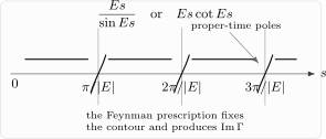
The in-out contour $\mathcal C_+$ bypasses $s_n=n\pi/E$ above the positive real axis. The enlarged upper semicircle contributes $-i\pi R_n$ for residue $R_n$. Combined with the scalar or spinor prefactor, this gives positive $\operatorname{Im}\mathcal L_M^{(1)}$. Distances and indentation radii are schematic; the poles and orientation are exact. This is a contour in complex proper time, not a graph of the integrand.

To check the sign, write $s=s_n+\rho e^{i\theta}$ with $\theta$ decreasing from $\pi$ to $0$. A simple pole contributes $\int iR_n\,d\theta=-i\pi R_n$. Including all prefactors, the residues are

$$R_{s,n}=\frac{(-1)^n e^{-m^2s_n}}{16\pi^2s_n^2},\qquad R_{f,n}=-\frac{e^{-m^2s_n}}{8\pi^2s_n^2}.$$

Consequently,

$$\begin{aligned} \operatorname{Im}\mathcal L_{M,s}^{(1)} &=\frac{E^2}{16\pi^3}\sum_{n=1}^\infty \frac{(-1)^{n+1}}{n^2}e^{-n\pi m^2/E},\\ \operatorname{Im}\mathcal L_{M,f}^{(1)} &=\frac{E^2}{8\pi^3}\sum_{n=1}^\infty \frac1{n^2}e^{-n\pi m^2/E}. \end{aligned}$$

Both are positive; the scalar sum is alternating with decreasing term magnitude. They agree with Dunne 2004, Eqs. (1.25) and (1.37), PDF pp. 12 and 14. Reversing the contour would give the unphysical vacuum-growth sign for these conventions.

For a prescribed uniform field in the large-volume, long-time limit,

$$\langle0_{\rm out}|0_{\rm in}\rangle_A=e^{i\Gamma_M[A]},\qquad P_{\rm vac}=e^{-2\operatorname{Im}\Gamma_M[A]},\qquad -\frac{\log P_{\rm vac}}{VT}=2\operatorname{Im}\mathcal L_M.$$

This is the vacuum-decay exponent per volume and time, with backreaction neglected. It is not in general the mean pair-number production rate; those coincide at leading dilute-pair order. Nor is this in-out quantity a retarded response kernel. The exponentially small electric instability is invisible at every fixed order of the real weak-field series.

For weak slowly varying fields, after the $F^2$ term is renormalized, the remaining local effective action begins with fourth-order invariants. In Minkowski notation these are built from

$$\mathcal F={1\over2}(\mathbf B^2-\mathbf E^2), \qquad \mathcal G=\mathbf E\cdot\mathbf B.$$

The precise coefficients depend on the spin and charge of the particle in the loop. Their existence is the important structural point: integrating out massive charged matter produces local nonlinear photon interactions at energies small compared with the mass.

Summary

A one-loop effective action in a background field is a determinant. Proper time turns that determinant into a heat-kernel trace. For a constant magnetic field, the heat kernel is exactly computable because the transverse motion is a Landau-level problem.

For a complex scalar in four dimensions,

$${1\over V_4}\operatorname{Tr}e^{-s(-D^2)} ={1\over(4\pi s)^2}{Bs\over\sinh Bs},$$

and the logarithmic $B^2$ term gives

$$\Delta\left({1\over e^2}\right)_s ={1\over16\pi^2}{1\over3}\log {\Lambda^2\over m^2}.$$

For a Dirac fermion,

$${1\over V_4}\operatorname{Tr}e^{-s[-(\gamma_\mu D_\mu)^2]} ={4\over(4\pi s)^2}Bs\coth Bs,$$

and

$$\Delta\left({1\over e^2}\right)_f ={1\over16\pi^2}{4\over3}\log {\Lambda^2\over m^2}.$$

The scalar result comes from orbital Landau motion. The spinor result is larger because the spin magnetic moment contributes a paramagnetic term. These positive shifts of $1/e^2$ are cutoff matching statements; when translated into the running of $e(\mu)$, they give the familiar positive QED beta function. The background-field method generalizes this logic to Yang–Mills theory, where spin-one gauge fluctuations produce the antiscreening sign.

After subtracting the vacuum and $F^2$ terms, the constant-field proper-time integrals are finite. Their expansion begins at $B^4/m^4$ and gives the low-energy nonlinear photon interactions encoded by the Euler–Heisenberg action.

Common pitfalls

Proper time is not inverse temperature. Both $s$ and $\beta$ appear in traces and can produce hyperbolic functions, but $s$ is a spectral parameter while $\beta$ is the circumference of the physical Euclidean-time circle.

An ordinary momentum cutoff is not gauge covariant in a general background. A proper-time cutoff regulates the spectrum of a covariant operator and organizes divergences into gauge-invariant local terms.

The unrenormalized $F^2$ coefficient is not a finite prediction. It renormalizes the gauge coupling. The higher-dimension terms left after the vacuum and $F^2$ subtractions are finite low-energy matching data.

Gauge-field normalization changes displayed coefficients. Some references keep $e$ in $D_\mu=\partial_\mu-ieA_\mu$ and write $F^2/4$. Here the background is rescaled so the kinetic term contains $1/e^2$ and positively charged unit matter couples through $D_\mu=\partial_\mu-iA_\mu$.

Squaring the Dirac operator does not erase spin. Dropping the Pauli term turns a spinor into several scalar-like degrees of freedom and gives the wrong coefficient. The determinant phase must also be retained when parity-odd terms or anomalies are in scope.

Hermitian and anti-Hermitian connection notation must not be mixed silently. The Abelian sections use $D=\partial-iA$ with Hermitian $A$. The background-field-gauge preview writes $\mathcal A=-iA^aT^a$ so that $\mathcal D=\partial+\mathcal A$ is the same derivative in anti-Hermitian notation; its connection transforms with $+g^{-1}\partial g$.

Exercises

Exercise 1: Derive the scalar magnetic heat kernel

Derive the scalar heat kernel in a constant magnetic field,

$${1\over V_4}\operatorname{Tr}e^{-s(-D^2)} ={1\over(4\pi s)^2}{Bs\over\sinh Bs}.$$

Use the Landau-level spectrum and degeneracy.

Solution

For $F_{12}=B$, the transverse eigenvalues are

$$(2n+1)B, \qquad n=0,1,2,\ldots,$$

with degeneracy per transverse area

$${B\over2\pi}.$$

The two directions parallel to the magnetic field are free, so

$${1\over V_4}\operatorname{Tr}e^{-s(-D^2)} = {B\over2\pi}\sum_{n=0}^\infty e^{-s(2n+1)B} \int {d^2p\over(2\pi)^2}e^{-sp^2}.$$

The free Gaussian integral is

$$\int {d^2p\over(2\pi)^2}e^{-sp^2}={1\over4\pi s}.$$

The Landau-level sum is

$$\sum_{n=0}^\infty e^{-s(2n+1)B} ={e^{-Bs}\over1-e^{-2Bs}} ={1\over2\sinh Bs}.$$

Combining these factors gives

$${B\over2\pi}\cdot {1\over2\sinh Bs}\cdot {1\over4\pi s} ={B\over16\pi^2s\sinh Bs} ={1\over(4\pi s)^2}{Bs\over\sinh Bs}.$$

Exercise 2: Match the scalar contribution to the Maxwell term

Using

$${x\over\sinh x}=1-{x^2\over6}+O(x^4),$$

extract the logarithmic scalar contribution to $1/e^2$.

Solution

The scalar effective action is

$${\Gamma_s^{(1)}[B]-\Gamma_s^{(1)}[0]\over V_4} = -\int_\epsilon^\infty {ds\over s}\,e^{-m^2s} {1\over(4\pi s)^2} \left({Bs\over\sinh Bs}-1\right).$$

Using the expansion,

$${Bs\over\sinh Bs}-1=-{B^2s^2\over6}+O(B^4s^4).$$

Thus

$${\Gamma_s^{(1)}[B]\over V_4} \supset {B^2\over6(4\pi)^2} \int_\epsilon^\infty {ds\over s}e^{-m^2s}.$$

The logarithmic part is

$$\int_\epsilon^\infty {ds\over s}e^{-m^2s} = \log {\Lambda^2\over m^2}+\text{finite}.$$

Therefore

$$\Gamma_s^{(1)}[B] \supset {V_4B^2\over96\pi^2}\log {\Lambda^2\over m^2}.$$

Since

$$V_4B^2={1\over2}\int d^4x\,F_{\mu\nu}F_{\mu\nu},$$

we have

$$\Gamma_s^{(1)}[A] \supset {1\over192\pi^2}\log {\Lambda^2\over m^2} \int d^4x\,F_{\mu\nu}F_{\mu\nu}.$$

Matching to

$${1\over4}\Delta\left({1\over e^2}\right) \int d^4x\,F_{\mu\nu}F_{\mu\nu}$$

gives

$$\Delta\left({1\over e^2}\right)_s ={1\over48\pi^2}\log {\Lambda^2\over m^2} ={1\over16\pi^2}{1\over3}\log {\Lambda^2\over m^2}.$$

Exercise 3: Separate orbital and spin contributions in QED

Show that the spinor heat-kernel factor produces the coefficient $4/3$ in spinor QED. More precisely, use

$$4x\coth x=4{x\over\sinh x}\cosh x$$

and expand to order $x^2$.

Solution

The two factors have small-$x$ expansions

$${x\over\sinh x}=1-{x^2\over6}+O(x^4),$$

and

$$\cosh x=1+{x^2\over2}+O(x^4).$$

Therefore

$$4{x\over\sinh x}\cosh x =4\left(1-{x^2\over6}+O(x^4)\right) \left(1+{x^2\over2}+O(x^4)\right).$$

Multiplying gives

$$4{x\over\sinh x}\cosh x =4\left(1+\left[-{1\over6}+{1\over2}\right]x^2+O(x^4)\right).$$

Hence

$$4{x\over\sinh x}\cosh x =4\left(1+{x^2\over3}+O(x^4)\right) =4+{4\over3}x^2+O(x^4).$$

The orbital part contributes

$$4\left(-{1\over6}\right)=-{2\over3},$$

while the spin factor contributes

$$4\left({1\over2}\right)=2.$$

Their sum is

$$-{2\over3}+2={4\over3}.$$

This is the coefficient that leads to

$$\Delta\left({1\over e^2}\right)_f ={1\over16\pi^2}{4\over3}\log {\Lambda^2\over m^2}.$$

Exercise 4: Verify background-gauge covariance

Let

$$\mathcal A_\mu=\overline{\mathcal A}_\mu+a_\mu.$$

Under a background gauge transformation,

$$\overline{\mathcal A}_\mu \mapsto g^{-1}\overline{\mathcal A}_\mu g+g^{-1}\partial_\mu g, \qquad a_\mu\mapsto g^{-1}a_\mu g.$$

Show that $\overline{\mathcal D}_\mu a_\nu$ transforms homogeneously.

Solution

The background covariant derivative is

$$\overline{\mathcal D}_\mu a_\nu =\partial_\mu a_\nu+[\overline{\mathcal A}_\mu,a_\nu].$$

A compact way to prove the transformation law is to let it act on an adjoint test field $X$, which transforms as

$$X\mapsto X'=g^{-1}Xg.$$

The transformed background derivative is

$$\overline{\mathcal D}'_\mu X' =\partial_\mu(g^{-1}Xg) +[g^{-1}\overline{\mathcal A}_\mu g+g^{-1}\partial_\mu g,g^{-1}Xg].$$

Using

$$\partial_\mu g^{-1}=-g^{-1}(\partial_\mu g)g^{-1},$$

the terms involving $\partial_\mu g$ cancel, leaving

$$\overline{\mathcal D}'_\mu X' =g^{-1}(\partial_\mu X+[\overline{\mathcal A}_\mu,X])g =g^{-1}(\overline{\mathcal D}_\mu X)g.$$

Taking $X=a_\nu$ gives

$$\boxed{ \overline{\mathcal D}'_\mu a'_\nu =g^{-1}(\overline{\mathcal D}_\mu a_\nu)g. }$$

Thus the background gauge condition $\overline{\mathcal D}_\mu a_\mu=0$ is covariant under background gauge transformations.

Exercise 5: Locate the electric-field proper-time poles

Explain why $B\to-i(E+i0)$ changes $Bs/\sinh Bs$ into $Es/\sin Es$, identify the pole locations and their side of approach, and check the imaginary contribution of the first pole to the scalar loop Lagrangian. Would changing only $m^2$ in the Euclidean exponential determine that contribution?

Solution

Using

$$\sinh(-iEs)=-i\sin(Es),$$

we find

$${Bs\over\sinh Bs}\bigg|_{B=-iE} ={-iEs\over\sinh(-iEs)} ={-iEs\over-i\sin(Es)} ={Es\over\sin(Es)}.$$

The denominator vanishes when

$$\sin(Es)=0,$$

so the positive real proper-time poles are at

$$\boxed{ s_n={n\pi\over E}, \qquad n=1,2,\ldots. }$$

Before the limit, $B=\eta-iE$ with $\eta>0$ puts each positive pole at $s_n=-in\pi/(\eta-iE)$ below the real axis. The limiting contour therefore passes above it. Near $s_1=\pi/E$, $\sin(Es)=-E(s-s_1)+O((s-s_1)^3)$, so the residue of the full scalar integrand is

$$R_{s,1}=-\frac{e^{-m^2s_1}}{16\pi^2s_1^2}.$$

The upper, clockwise indentation contributes $-i\pi R_{s,1}$, hence

$$\left(\operatorname{Im}\mathcal L_{M,s}^{(1)}\right)_{n=1} =\frac{E^2}{16\pi^3}e^{-\pi m^2/E}>0.$$

Changing only $m^2$ in $e^{-m^2s}$ leaves the sine zeros fixed, so it cannot choose a bypass. The field continuation and contour are necessary parts of the in-out definition.

References

• Dunne, Gerald V. “Heisenberg–Euler Effective Lagrangians: Basics and Extensions.” In From Fields to Strings: Circumnavigating Theoretical Physics, vol. 1, 445–522. World Scientific, 2005. DOI. Cited preprint: arXiv:hep-th/0406216v1, 2004. Open PDF.
• Schwartz, Matthew D. Quantum Field Theory and the Standard Model. Cambridge University Press, 2014. DOI.
• Schwinger, Julian. “On Gauge Invariance and Vacuum Polarization.” Physical Review 82, no. 5 (1951): 664–679. DOI. Open publisher PDF.

Further reading

• Heisenberg, Werner, and Hans Euler. “Folgerungen aus der Diracschen Theorie des Positrons.” Zeitschrift für Physik 98 (1936): 714–732.
• Srednicki, Mark. Quantum Field Theory. Cambridge University Press, 2007.
• Weinberg, Steven. The Quantum Theory of Fields, Volume II: Modern Applications. Cambridge University Press, 1996.
• Zee, A. Quantum Field Theory in a Nutshell. 2nd ed. Princeton University Press, 2010.
• Zinn-Justin, Jean. Quantum Field Theory and Critical Phenomena. 4th ed. Oxford University Press, 2002.