Vector Fields and Gauge Redundancy

Spin-zero and spin-one-half fields can be quantized without introducing an obvious redundancy in the field variables. Vector fields are different. A massive vector field has three physical polarizations, and the Proca equation enforces this by a constraint. A massless vector field, however, has only two physical helicities. If we insist on using a Lorentz four-vector $A_\mu(x)$ to describe those two helicities, we have necessarily introduced more variables than physical degrees of freedom.

This is the origin of gauge redundancy. The Maxwell field is not merely a vector field with $m=0$. It is a vector field whose physically meaningful content is invariant under

$$A_\mu(x)\longmapsto A_\mu(x)+\partial_\mu\alpha(x).$$

The redundancy is not an optional decoration. It is what makes a local Lorentz-covariant description of massless spin one possible, and it is the reason conserved currents, covariant derivatives, Ward identities, and gauge fixing all enter QFT together.

There are three statements to keep separate throughout the page. First, $A_\mu$ is a Lorentz four-vector field. Second, a photon is a massless spin-one particle with two helicities. Third, a gauge choice is a representative of a redundant description, not an observable. Many mistakes in gauge theory come from treating these three statements as if they were the same.

Required background. Scalar and vector representations and mass shells supplies the Lorentz-representation and polarization language used below. Helpful background. Dirac fields and spinors supplies the on-shell spinor identities used when matter is introduced.

Massive vector fields and the Proca constraint

A Lorentz vector field transforms as

$$A'^\mu(x')=\Lambda^\mu{}_{\nu}A^\nu(x), \qquad x'=\Lambda x.$$

As a field representation this has four components. A massive spin-one particle, however, has only three spin states. The Proca Lagrangian implements the required reduction:

$$\mathcal L_{\mathrm{Proca}} =-{1\over4}F_{\mu\nu}F^{\mu\nu} +{1\over2}M^2A_\mu A^\mu, \qquad F_{\mu\nu}=\partial_\mu A_\nu-\partial_\nu A_\mu.$$

Varying $A_\nu$ gives

$$\partial_\mu F^{\mu\nu}+M^2A^\nu=0.$$

Taking the divergence gives

$$\partial_\nu\partial_\mu F^{\mu\nu}+M^2\partial_\nu A^\nu=0.$$

The first term vanishes because $F^{\mu\nu}$ is antisymmetric while $\partial_\nu\partial_\mu$ is symmetric. Therefore, for $M\neq0$,

$$\partial_\mu A^\mu=0.$$

Substituting this back into the equation of motion gives

$$(\partial^2+M^2)A^\nu=0.$$

For a plane wave

$$A^\mu(x)=\epsilon^\mu(p)e^{-ip\cdot x},$$

the equations become

$$p^2=M^2, \qquad p_\mu\epsilon^\mu(p)=0.$$

The second condition is the Proca transversality constraint. It removes one of the four components of $\epsilon^\mu$, leaving three physical polarizations.

This condition is an equation-of-motion constraint, not a gauge choice. The mass term removes the Maxwell gauge redundancy: for $M\neq0$, two Proca configurations that differ by $\partial_\mu\alpha$ are generally physically different. In Hamiltonian language $A_0$ has no independent second-order evolution equation; eliminating it leaves three propagating canonical modes.

In the rest frame $p^\mu=(M,0,0,0)$, the condition $p\cdot\epsilon=0$ gives

$$M\epsilon^0=0,$$

so $\epsilon^0=0$. The remaining three components are an ordinary spatial vector. A convenient basis is

$$\epsilon_1^\mu=(0,1,0,0), \qquad \epsilon_2^\mu=(0,0,1,0), \qquad \epsilon_3^\mu=(0,0,0,1).$$

Thus the Proca field contains precisely the spin-one representation of the massive little group $SO(3)$.

The massive polarization sum is

$$\sum_{\lambda=1}^{3} \epsilon_\lambda^\mu(p)\epsilon_\lambda^{*\nu}(p) =-\eta^{\mu\nu}+{p^\mu p^\nu\over M^2},$$

where the physical polarizations are normalized by

$$\epsilon_\lambda^*(p)\cdot\epsilon_{\lambda'}(p)=-\delta_{\lambda\lambda'}.$$

The polarization sum on the right is singular as $M\to0$. As a mixed-index map $C^\mu{}_\nu$, it satisfies $C^2=-C$; the idempotent projection onto $p^\perp$ is $T=-C$. This distinction and the conjugation needed for a complex basis were derived in lesson 32 and the canonical polarization treatment. The singularity warns that the massless limit requires separate control of the longitudinal mode.

The same polarization tensor appears in the free Proca propagator,

$$D^{\mathrm P}_{\mu\nu}(p) ={-i\over p^2-M^2+i\epsilon} \left(\eta_{\mu\nu}-{p_\mu p_\nu\over M^2}\right).$$

Unlike the photon propagator below, this is not part of a one-parameter family of gauges: the Proca kinetic operator is invertible for $M\neq0$. The $p_\mu p_\nu/M^2$ term records a physical longitudinal polarization rather than a redundant gauge direction.

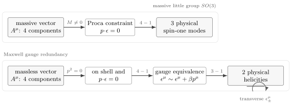
A massive vector has four components minus the Proca constraint $p\cdot\epsilon=0$, leaving three polarizations. A massless vector has the on-shell condition $p^2=0$, transversality, and the gauge equivalence $\epsilon^\mu\sim\epsilon^\mu+\beta p^\mu$, leaving two helicities.

The longitudinal mode and conserved currents

The apparent singularity in the massive polarization sum is associated with the longitudinal polarization. For momentum $p^\mu=(E,0,0,|\mathbf p|)$, one convenient longitudinal massive polarization is

$$\epsilon_L^\mu(p)={1\over M}(|\mathbf p|,0,0,E).$$

It obeys

$$p\cdot\epsilon_L=E{|\mathbf p|\over M}-|\mathbf p|{E\over M}=0,$$

and

$$\epsilon_L^2=-1.$$

Take $M\to0$ at fixed $|\mathbf p|>0$. Then $E\sim|\mathbf p|$, so

$$\epsilon_L^\mu(p)={p^\mu\over M}+O(M).$$

If the vector field couples to a current matrix element $J_\mu$ whose components stay bounded in this limit, the longitudinal contribution contains

$$\epsilon_L^\mu J_\mu ={1\over M}p^\mu J_\mu+O(M).$$

For a conserved current,

$$p_\mu J^\mu=0.$$

Therefore the dangerous $1/M$ part vanishes. More explicitly, conservation gives $EJ^0=|\mathbf p|J^3$, hence $\epsilon_L\cdot J=-MJ^3/E$. This vanishes for the bounded current at fixed nonzero momentum. Conservation alone does not bound a family of current matrix elements as a parameter changes; the stated regularity is essential to this decoupling argument.

This statement is often the cleanest way to remember what gauge invariance is doing. The massless photon has no longitudinal physical polarization. Coupling it consistently to matter requires amplitudes to be insensitive to adding a multiple of $p^\mu$ to the polarization vector. Current conservation is the corresponding condition on the matter side.

Maxwell theory

Set the vector mass to zero and keep only the field-strength term:

$$\mathcal L_{\mathrm{Maxwell}} =-{1\over4}F_{\mu\nu}F^{\mu\nu}.$$

For redundancy statements, work on topologically trivial Minkowski space and restrict to proper gauge transformations, for example smooth gauge functions of compact support, or boundary falloff that gives zero boundary charge. Transformations with nontrivial boundary charges require a separate physical-symmetry analysis. The canonical Maxwell treatment explains this boundary distinction.

This Lagrangian is invariant under

$$A_\mu\mapsto A_\mu+\partial_\mu\alpha.$$

Indeed,

$$F_{\mu\nu}\mapsto \partial_\mu(A_\nu+\partial_\nu\alpha) -\partial_\nu(A_\mu+\partial_\mu\alpha) =F_{\mu\nu},$$

because mixed partial derivatives commute. The field strength, not the potential itself, is gauge invariant.

Denote the Maxwell source current by $J_{\mathrm{source}}^\mu$ and choose the source coupling

$$\mathcal L_{\mathrm{source}}=-J_{\mathrm{source}}^\mu A_\mu,$$

the Euler–Lagrange equation is

$$\partial_\mu F^{\mu\nu}=J_{\mathrm{source}}^\nu.$$

The divergence of the left side vanishes identically:

$$\partial_\nu\partial_\mu F^{\mu\nu}=0.$$

Therefore consistency requires

$$\partial_\nu J_{\mathrm{source}}^\nu=0.$$

The same condition follows from gauge invariance of the coupling to matter. The source action is

$$S_{\mathrm{int}}=-\int d^4x\,J_{\mathrm{source}}^\mu A_\mu.$$

Under $A_\mu\mapsto A_\mu+\partial_\mu\alpha$,

$$\delta S_{\mathrm{int}} =-\int d^4x\,J_{\mathrm{source}}^\mu\partial_\mu\alpha =\int d^4x\,\alpha\,\partial_\mu J_{\mathrm{source}}^\mu,$$

up to a boundary term. For arbitrary $\alpha(x)$, this vanishes only if

$$\partial_\mu J_{\mathrm{source}}^\mu=0.$$

The logic can be read in either direction. If a theory has a conserved current, it can couple naturally to a massless vector field. If a massless vector field couples consistently to matter, gauge redundancy forces the current seen by the vector field to be conserved.

In vacuum, a plane wave obeys $p^2=0$ and may be represented by a polarization satisfying $p\cdot\epsilon=0$. The latter condition still leaves three components because a null vector is orthogonal to itself. The residual equivalence

$$\epsilon_\mu\sim\epsilon_\mu+\beta p_\mu$$

removes one more component, leaving two helicities. This is different from Proca theory twice over: in Maxwell theory $\partial\cdot A=0$ is imposed as a convenient Lorenz gauge condition rather than obtained as a Proca constraint, and the remaining longitudinal shift is a redundancy rather than a physical mode.

Why naive Lorentz-covariant quantization fails

One might try to quantize the four components of $A_\mu$ as if they were four scalar fields. This immediately produces trouble. A Lorentz-covariant oscillator algebra has the schematic form

$$[a_\mu(\mathbf p),a_\nu^\dagger(\mathbf q)] =-(2\pi)^3 2E_{\mathbf p}\,\eta_{\mu\nu}\delta^{(3)}(\mathbf p-\mathbf q).$$

The spatial components then have positive norm because $-\eta_{ij}=\delta_{ij}$, but the time component has

$$[a_0(\mathbf p),a_0^\dagger(\mathbf q)] =-(2\pi)^3 2E_{\mathbf p}\delta^{(3)}(\mathbf p-\mathbf q).$$

Thus the one-particle state $a_0^\dagger|0\rangle$ has negative norm:

$$\langle0|a_0a_0^\dagger|0\rangle<0.$$

A Hilbert space with negative-norm physical states is unacceptable. Gauge theory avoids this conclusion by telling us that not all components of $A_\mu$ create physical states. The timelike and longitudinal modes are artifacts of the Lorentz-covariant description.

This is not just a minor bookkeeping problem. The Maxwell quadratic action can be written, after integrating by parts, as

$$S_0={1\over2}\int d^4x\, A_\mu\left(\eta^{\mu\nu}\partial^2-\partial^\mu\partial^\nu\right)A_\nu.$$

In momentum space the kinetic operator is proportional to

$$K^{\mu\nu}(p)=-p^2\eta^{\mu\nu}+p^\mu p^\nu,$$

where the sign follows from the course convention $\partial_\mu\mapsto-ip_\mu$. It has a zero mode:

$$K^{\mu\nu}(p)p_\nu=0.$$

The zero mode is exactly the gauge direction $A_\mu(p)\sim A_\mu(p)-ip_\mu\alpha(p)$, obtained by Fourier transforming $A_\mu\mapsto A_\mu+\partial_\mu\alpha$. Therefore the kinetic operator is not invertible until we fix a gauge or otherwise remove the redundant directions.

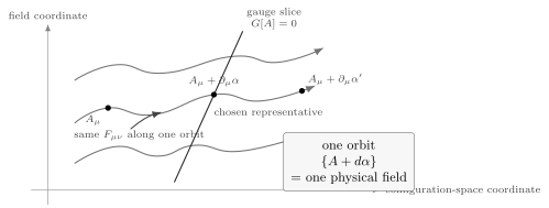
The figure is a local schematic for the admitted proper gauge transformations. A gauge condition selects representatives, with boundary data and any residual transformations still to be fixed; it is not a theorem that an arbitrary gauge condition intersects every orbit exactly once. Potentials along such a proper orbit describe the same physical configuration.

Gauge fixing and photon propagators

To calculate with a photon propagator, we need an inverse kinetic operator with specified boundary data. A Lorenz condition still admits residual transformations satisfying $\Box\alpha=0$; the vacuum prescription and remaining boundary restrictions must handle them. One standard Lorentz-covariant choice adds the gauge-fixing term

$$\mathcal L_{\mathrm{gf}} =-{1\over2\xi}(\partial_\mu A^\mu)^2.$$

For $\xi\neq0$ the quadratic operator is

$$K^{(\xi)}_{\mu\nu}(p) =-p^2\eta_{\mu\nu} +\left(1-{1\over\xi}\right)p_\mu p_\nu,$$

with the overall sign fixed by $\mathcal L=-F^2/4-(\partial\cdot A)^2/(2\xi)$. Its inverse gives the momentum-space photon propagator

$$D_{\mu\nu}(p) ={-i\over p^2+i\epsilon} \left[ \eta_{\mu\nu}-(1-\xi){p_\mu p_\nu\over p^2} \right].$$

The pole prescription in the longitudinal term is understood as the corresponding limit of the gauge-fixed inverse; writing a second $p^2+i\epsilon$ there is an equivalent common shorthand. In Feynman gauge, $\xi=1$, this simplifies to

$$D_{\mu\nu}(p)={-i\eta_{\mu\nu}\over p^2+i\epsilon}.$$

This expression propagates four components, but only gauge-invariant combinations are observable. Between conserved currents, the gauge-dependent term is proportional to

$$(p\cdot J_1)(p\cdot J_2)=0,$$

so the exchange amplitude is independent of $\xi$. In Abelian gauge theory the Faddeev–Popov determinant for a linear covariant gauge is field independent, so its ghosts decouple. In non-Abelian gauge theory the determinant depends on the gauge field, and ghost loops are essential. For the present QFT I discussion, the main point is simpler: the propagator exists only after the redundant gauge directions are handled.

Different gauges emphasize different virtues. Lorenz-type gauges preserve manifest Lorentz covariance. Coulomb gauge, $\nabla\cdot\mathbf A=0$, displays the two transverse photon polarizations more directly but hides manifest covariance. Temporal gauge, $A_0=0$, is sometimes intuitive but leaves residual gauge freedom. Physical answers must be independent of this choice.

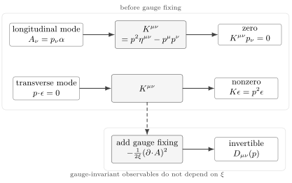
The Maxwell kinetic operator annihilates longitudinal modes proportional to $p_\mu$. This is why the free Maxwell quadratic form cannot be inverted before gauge fixing. Gauge fixing lifts the degeneracy of the quadratic form without changing gauge-invariant observables.

Local phase symmetry and the covariant derivative

Now suppose a matter theory has a global $U(1)$ symmetry. For a Dirac field,

$$\mathcal L_0=\bar\psi(i\gamma^\mu\partial_\mu-m)\psi$$

is invariant under

$$\psi\mapsto e^{iq\alpha}\psi, \qquad \bar\psi\mapsto \bar\psi e^{-iq\alpha},$$

when $\alpha$ is constant. If $\alpha$ depends on spacetime, then

$$\partial_\mu\psi\mapsto \partial_\mu(e^{iq\alpha}\psi) =e^{iq\alpha}\left(\partial_\mu\psi+iq(\partial_\mu\alpha)\psi\right).$$

The extra term prevents $\partial_\mu\psi$ from transforming like $\psi$. Introduce a vector field $A_\mu$ and define

$$D_\mu\psi=(\partial_\mu-iqA_\mu)\psi.$$

If

$$A_\mu\mapsto A_\mu+\partial_\mu\alpha,$$

then

$$D_\mu\psi\mapsto e^{iq\alpha}D_\mu\psi.$$

Thus a locally invariant Dirac Lagrangian is

$$\mathcal L=\bar\psi(i\gamma^\mu D_\mu-m)\psi -{1\over4}F_{\mu\nu}F^{\mu\nu}.$$

Expanding the covariant derivative gives

$$\bar\psi i\gamma^\mu D_\mu\psi =\bar\psi i\gamma^\mu\partial_\mu\psi +q\bar\psi\gamma^\mu\psi A_\mu.$$

Begin with the conserved Dirac bilinear

$$j_{\mathrm{bil}}^\mu=\bar\psi\gamma^\mu\psi.$$

The interaction and source conventions define two related charge-weighted currents. The covariant derivative above gives

$$\mathcal L_{\mathrm{int}} =qA_\mu j_{\mathrm{bil}}^\mu =A_\mu j_q^\mu, \qquad j_q^\mu=qj_{\mathrm{bil}}^\mu.$$

Relative to the earlier convention $\mathcal L_{\mathrm{source}}=-J_{\mathrm{source}}\!\cdot A$, the current on the right-hand side of Maxwell’s equation is therefore

$$J_{\mathrm{source}}^\mu=-j_q^\mu =-qj_{\mathrm{bil}}^\mu.$$

Thus a positive $q$ gives the Lorentzian interaction $+qA_\mu j_{\mathrm{bil}}^\mu$. For an electron, $q=-e$, so the interaction is $-eA_\mu j_{\mathrm{bil}}^\mu$ and the vertex is $-ie\gamma^\mu$. Keeping the labels distinct prevents the sign in the vertex coefficient from being mistaken for the sign in the convention $-J_{\mathrm{source}}\!\cdot A$.

The scalar version is similar. For a complex scalar field of charge $q$,

$$\mathcal L=(D_\mu\phi)^*(D^\mu\phi)-m^2\phi^*\phi -{1\over4}F_{\mu\nu}F^{\mu\nu}.$$

Here the star matters:

$$(D_\mu\phi)^* =(\partial_\mu+iqA_\mu)\phi^*.$$

Thus the conjugate field carries the opposite charge. A common alternative is to absorb the charge into the gauge potential. Define

$$\mathcal A_\mu=qA_\mu, \qquad \mathcal D_\mu=\partial_\mu-i\mathcal A_\mu.$$

Then

$$(\mathcal D_\mu\phi)^*(\mathcal D^\mu\phi) =(\partial_\mu+i\mathcal A_\mu)\phi^* (\partial^\mu-i\mathcal A^\mu)\phi.$$

If the kinetic term for the rescaled gauge field is written with the coupling outside, the Lagrangian becomes schematically

$$\mathcal L=(\mathcal D_\mu\phi)^*(\mathcal D^\mu\phi) -m^2|\phi|^2-{1\over4q^2}\mathcal F_{\mu\nu}\mathcal F^{\mu\nu}.$$

The placement of the coupling is a convention; the opposite signs on the two conjugate scalar factors are not. They are required because $\phi^*$ has charge $-q$ when $\phi$ has charge $q$.

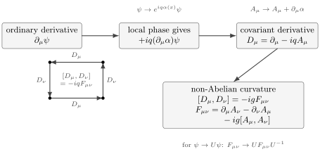
A local phase rotation makes ordinary derivatives transform inhomogeneously. The gauge field $A_\mu$ supplies the connection term in $D_\mu$. The field strength $F_{\mu\nu}$ is the curvature: it measures the phase accumulated around an infinitesimal loop.

Field strength as a commutator

The field strength can be characterized without guessing its formula. For the Abelian covariant derivative

$$D_\mu=\partial_\mu-iqA_\mu,$$

the commutator is

$$[D_\mu,D_\nu] =-iq(\partial_\mu A_\nu-\partial_\nu A_\mu) =-iqF_{\mu\nu}.$$

Thus $F_{\mu\nu}$ is the obstruction to commuting two covariant derivatives. Geometrically, $A_\mu$ is a connection and $F_{\mu\nu}$ is its curvature.

This viewpoint generalizes immediately, but the sign bookkeeping is slightly less forgiving. With Hermitian generators and $D_\mu=\partial_\mu-igA_\mu^aT^a$, the non-Abelian field strength contains a plus sign in components, $F_{\mu\nu}^a=\partial_\mu A_\nu^a-\partial_\nu A_\mu^a+gf^{abc}A_\mu^bA_\nu^c$. In matrix notation this same statement is cleaner. Let $U(x)=e^{ig\alpha^a(x)T^a}$ and let $\psi$ transform in a representation of a non-Abelian group $G$:

$$\psi(x)\mapsto U(x)\psi(x), \qquad U(x)\in G.$$

Write the gauge field as a matrix

$$A_\mu=A_\mu^aT^a, \qquad [T^a,T^b]=if^{abc}T^c,$$

and define

$$D_\mu=\partial_\mu-igA_\mu.$$

The gauge field must transform so that

$$D_\mu\psi\mapsto U(D_\mu\psi).$$

Equivalently,

$$D_\mu\mapsto UD_\mu U^{-1}.$$

This gives

$$A_\mu\mapsto U A_\mu U^{-1}-{i\over g}(\partial_\mu U)U^{-1}.$$

The field strength is defined by

$$[D_\mu,D_\nu]=-igF_{\mu\nu},$$

so

$$F_{\mu\nu} =\partial_\mu A_\nu-\partial_\nu A_\mu-ig[A_\mu,A_\nu].$$

The commutator term is the new feature of Yang–Mills theory. Since $[T^a,T^b]=if^{abc}T^c$, the displayed matrix formula gives

$$F_{\mu\nu}^a =\partial_\mu A_\nu^a-\partial_\nu A_\mu^a+gf^{abc}A_\mu^bA_\nu^c.$$

References that instead use $D_\mu=\partial_\mu+igA_\mu$ have the opposite sign in the commutator term. The defining equation $[D_\mu,D_\nu]=-igF_{\mu\nu}$ fixes the signs used here.

Under a gauge transformation,

$$F_{\mu\nu}\mapsto UF_{\mu\nu}U^{-1}.$$

Therefore $\operatorname{tr}(F_{\mu\nu}F^{\mu\nu})$ is gauge invariant, and the Yang–Mills action is

$$\mathcal L_{\mathrm{YM}} =-{1\over2}\operatorname{tr}(F_{\mu\nu}F^{\mu\nu}).$$

Here the trace is normalized by $\operatorname{tr}(T^aT^b)=\tfrac12\delta^{ab}$. For a trace in a representation with $\operatorname{tr}_R(T_R^aT_R^b)=T(R)\delta^{ab}$, the coefficient is $-1/[4T(R)]$.

For $U(1)$ the commutator vanishes and this reduces to Maxwell theory. For a non-Abelian group, the gauge bosons carry the gauge charge themselves, and the field strength contains cubic and quartic self-interactions after the action is expanded.

Ward identities from replacing a polarization by momentum

For an external photon with momentum $q$, a gauge transformation shifts a plane-wave polarization by

$$\epsilon_\mu(q)\longmapsto \epsilon_\mu(q)+\beta q_\mu.$$

A physical scattering amplitude cannot change under this replacement. If the amplitude with the external photon removed is written as $\mathcal M^\mu$, then

$$\mathcal M=\epsilon_\mu\mathcal M^\mu.$$

Gauge invariance requires

$$q_\mu\mathcal M^\mu=0.$$

This is the simplest form of a Ward identity.

For example, the scalar QED three-point vertex for a scalar of charge $Q$ is proportional to

$$+iQ(p_1+p_2)_\mu,$$

where the incoming photon momentum is $k=p_2-p_1$ with both scalar legs on shell. Replacing the photon polarization by $k_\mu$ gives the factor

$$k\cdot(p_1+p_2) =(p_2-p_1)\cdot(p_1+p_2) =p_2^2-p_1^2.$$

If the scalar particles have equal mass and are on shell,

$$p_1^2=p_2^2=m^2,$$

so

$$k\cdot(p_1+p_2)=0.$$

This small calculation contains the whole moral: the longitudinal piece of a photon polarization does not contribute to a physical amplitude. In the next page, this becomes a practical rule for QED vertices and tree amplitudes.

Gauge redundancy is not an ordinary global symmetry

It is tempting to speak of gauge invariance as a symmetry, and this language is standard. But one should remember that it is a special kind of symmetry. A global symmetry can act on physical states. Proper gauge redundancy maps one description of a physical configuration to another description of the same physical configuration; a boundary transformation carrying a nonzero charge is not included in this identification.

The difference is visible already in Maxwell theory. The field strength $F_{\mu\nu}$ is unchanged by

$$A_\mu\mapsto A_\mu+\partial_\mu\alpha.$$

Thus $A_\mu$ and $A_\mu+\partial_\mu\alpha$ cannot represent distinct measured electromagnetic fields. The physical observables must be gauge invariant, such as $F_{\mu\nu}$, Wilson loops, scattering amplitudes, or properly dressed charged operators.

This does not make gauge theory empty. Quite the opposite: the redundancy imposes strong constraints. It forbids a photon mass term $M^2A_\mu A^\mu/2$, requires matter to enter through covariant derivatives, enforces current conservation, constrains counterterms, and leads to Ward identities. In non-Abelian gauge theories, the same principle generates the self-interactions of gluons and underlies the structure of the Standard Model.

Summary

A massive vector field is described by the Proca equation. Its divergence gives the dynamical constraint $\partial_\mu A^\mu=0$, so a four-component Lorentz vector carries three physical spin-one polarizations. At fixed nonzero momentum, a conserved current matrix element that remains bounded as $M\to0$ decouples from the longitudinal polarization.

A massless vector field is described by Maxwell theory with the gauge redundancy $A_\mu\sim A_\mu+\partial_\mu\alpha$. The field strength $F_{\mu\nu}$ is invariant, and the free Maxwell kinetic operator has zero modes precisely along gauge directions. Gauge fixing is required to define a propagator, but physical quantities must be independent of the gauge choice.

Local phase invariance replaces ordinary derivatives by covariant derivatives. The field strength is the commutator of covariant derivatives. For Abelian gauge theory this gives $F_{\mu\nu}=\partial_\mu A_\nu-\partial_\nu A_\mu$; for non-Abelian gauge theory it adds a commutator term and hence gauge-boson self-interactions. The first practical consequence is the Ward identity: amplitudes vanish when an external photon polarization is replaced by its momentum.

Common pitfalls

Components are not polarizations. The covariant field $A_\mu$ has four components, but a photon has two physical helicities. Transversality and the gauge equivalence must both be used in the massless count.

The Proca constraint is not a gauge condition. For $M\neq0$, $\partial\cdot A=0$ follows from the equations of motion and the longitudinal polarization is physical. In Maxwell theory a Lorenz condition selects representatives of gauge orbits and does not create a third photon polarization.

Proper gauge transformations are redundancies. They identify descriptions of the same physical configuration. Transformations carrying boundary charges can instead act as physical symmetries; equality of the local field strength alone does not decide their status.

The Maxwell operator has no inverse before gauge fixing. Its zero modes are the gauge directions, not an algebraic accident. A propagator becomes well defined only after restricting or lifting those directions.

A bare vector mass breaks Maxwell gauge invariance. The term $M^2A_\mu A^\mu/2$ is not invariant by itself. Gauge-invariant massive-vector theories require additional structure, such as a Stueckelberg or Higgs field.

A sign convention is a package. With $D_\mu=\partial_\mu-iqA_\mu$ and $\psi\mapsto e^{iq\alpha}\psi$, the transformation of $A_\mu$, the matter vertex, and the conjugate derivative are fixed. In particular, $(D_\mu\phi)^*=(\partial_\mu+iqA_\mu)\phi^*$.

Exercises

Exercise 1

Derive the Proca constraint. Starting from

$$\partial_\mu F^{\mu\nu}+M^2A^\nu=0,$$

show that $\partial_\mu A^\mu=0$ for $M\neq0$, and then show that each component of $A^\mu$ obeys the Klein–Gordon equation.

Solution

Take $\partial_\nu$ of the Proca equation:

$$\partial_\nu\partial_\mu F^{\mu\nu}+M^2\partial_\nu A^\nu=0.$$

Since $F^{\mu\nu}=-F^{\nu\mu}$ and $\partial_\nu\partial_\mu$ is symmetric in $\mu,\nu$,

$$\partial_\nu\partial_\mu F^{\mu\nu}=0.$$

Therefore

$$M^2\partial_\nu A^\nu=0.$$

For $M\neq0$,

$$\partial_\nu A^\nu=0.$$

Now expand

$$\partial_\mu F^{\mu\nu} =\partial_\mu(\partial^\mu A^\nu-\partial^\nu A^\mu) =\partial^2A^\nu-\partial^\nu(\partial_\mu A^\mu).$$

Using $\partial_\mu A^\mu=0$, the equation becomes

$$(\partial^2+M^2)A^\nu=0.$$

Thus the Proca field is a massive Klein–Gordon field in each component, supplemented by the transversality constraint that removes one component.

Exercise 2

Show explicitly that the longitudinal Proca polarization decouples from a conserved current in the massless limit at fixed $|\mathbf p|>0$, assuming the current components remain bounded. Use

$$\epsilon_L^\mu(p)={1\over M}(|\mathbf p|,0,0,E), \qquad p^\mu=(E,0,0,|\mathbf p|),$$

with $E^2-\mathbf p^2=M^2$.

Solution

First check transversality:

$$p\cdot\epsilon_L =E{|\mathbf p|\over M}-|\mathbf p|{E\over M}=0.$$

The norm is

$$\epsilon_L^2={|\mathbf p|^2-E^2\over M^2}=-1.$$

For small $M$,

$$E=|\mathbf p|+{M^2\over2|\mathbf p|}+O(M^4),$$

so

$$\epsilon_L^\mu(p)={p^\mu\over M}+O(M).$$

The coupling to a current is

$$\epsilon_L^\mu J_\mu={1\over M}p^\mu J_\mu+O(M).$$

If the current is conserved, then in momentum space

$$p_\mu J^\mu=0.$$

The singular piece vanishes. In fact conservation gives $J^0=|\mathbf p|J^3/E$, so the exact contraction is $\epsilon_L\cdot J=-MJ^3/E$. Bounded $J^3$ therefore makes it vanish. As a negative control, $J^\mu=\epsilon_L^\mu/M$ is also transverse, but $\epsilon_L\cdot J=-1/M$ diverges. This family violates the bounded-current hypothesis and shows why conservation alone is insufficient.

Exercise 3

Let

$$K^{\mu\nu}(p)=-p^2\eta^{\mu\nu}+p^\mu p^\nu.$$

Show that $K^{\mu\nu}p_\nu=0$. Then add $\mathcal L_{\mathrm{gf}}=-(\partial\cdot A)^2/(2\xi)$, invert the resulting operator, and explain why its $\xi$-dependent part vanishes between conserved currents.

Solution

Compute

$$K^{\mu\nu}p_\nu =-p^2\eta^{\mu\nu}p_\nu+p^\mu p^\nu p_\nu.$$

Since $\eta^{\mu\nu}p_\nu=p^\mu$ and $p^\nu p_\nu=p^2$,

$$K^{\mu\nu}p_\nu =-p^2p^\mu+p^\mu p^2=0.$$

Thus $p_\nu$ is a null eigenvector of the kinetic operator. A matrix or differential operator with a null eigenvector has no inverse on the full vector space. Since a propagator is the inverse of the quadratic operator, the Maxwell propagator is undefined until one removes or lifts the gauge-zero directions by a gauge condition.

Introduce the transverse and longitudinal projectors

$$P^{\mathrm T}_{\mu\nu}=\eta_{\mu\nu}-{p_\mu p_\nu\over p^2}, \qquad P^{\mathrm L}_{\mu\nu}={p_\mu p_\nu\over p^2}.$$

The gauge-fixed operator is proportional to

$$-p^2\left(P^{\mathrm T}+{1\over\xi}P^{\mathrm L}\right),$$

so its Feynman inverse is

$$D_{\mu\nu}(p) ={-i\over p^2+i\epsilon} \left(P^{\mathrm T}_{\mu\nu}+\xi P^{\mathrm L}_{\mu\nu}\right) ={-i\over p^2+i\epsilon} \left[\eta_{\mu\nu}-(1-\xi){p_\mu p_\nu\over p^2}\right].$$

Contracting the last term with two currents gives a factor $(p\cdot J_1)(p\cdot J_2)$. It vanishes when both currents are conserved, proving that the exchange amplitude is independent of $\xi$.

Exercise 4

For scalar QED, the one-photon vertex for an incoming scalar momentum $p_1$ and outgoing scalar momentum $p_2$ is proportional to

$$(p_1+p_2)_\mu.$$

Let the photon momentum be $q=p_1-p_2$. Show that replacing the photon polarization by $q_\mu$ gives zero for equal-mass on-shell scalar particles.

Solution

The replacement gives the contraction

$$q\cdot(p_1+p_2).$$

Using $q=p_1-p_2$,

$$q\cdot(p_1+p_2) =(p_1-p_2)\cdot(p_1+p_2) =p_1^2-p_2^2.$$

For equal-mass on-shell scalar particles,

$$p_1^2=p_2^2=m^2.$$

Therefore

$$q\cdot(p_1+p_2)=0.$$

This is the tree-level Ward identity for the scalar three-point vertex.

Exercise 5

With

$$D_\mu=\partial_\mu-igA_\mu, \qquad A_\mu=A_\mu^aT^a,$$

define $F_{\mu\nu}$ by

$$[D_\mu,D_\nu]=-igF_{\mu\nu}.$$

Derive

$$F_{\mu\nu}=\partial_\mu A_\nu-\partial_\nu A_\mu-ig[A_\mu,A_\nu].$$

Solution

Let $D_\mu$ act on a test field $\psi$. Then

$$D_\mu D_\nu\psi =(\partial_\mu-igA_\mu)(\partial_\nu\psi-igA_\nu\psi).$$

Expanding,

$$D_\mu D_\nu\psi =\partial_\mu\partial_\nu\psi -ig(\partial_\mu A_\nu)\psi -igA_\nu\partial_\mu\psi -igA_\mu\partial_\nu\psi -g^2A_\mu A_\nu\psi.$$

Subtract the same expression with $\mu$ and $\nu$ exchanged. The second-derivative terms cancel, and so do the terms where a gauge field multiplies a derivative of $\psi$. The result is

$$[D_\mu,D_\nu]\psi =-ig(\partial_\mu A_\nu-\partial_\nu A_\mu)\psi -g^2(A_\mu A_\nu-A_\nu A_\mu)\psi.$$

This can be written as

$$[D_\mu,D_\nu]\psi =-ig\left(\partial_\mu A_\nu-\partial_\nu A_\mu-ig[A_\mu,A_\nu]\right)\psi.$$

Therefore

$$F_{\mu\nu}=\partial_\mu A_\nu-\partial_\nu A_\mu-ig[A_\mu,A_\nu].$$

For an Abelian group the commutator vanishes, recovering the Maxwell field strength.

Further reading

• Coleman, Sidney. Lectures of Sidney Coleman on Quantum Field Theory. Edited by Bryan Gin-ge Chen, David Derbes, David Griffiths, Brian Hill, Richard Sohn, and Yuan-Sen Ting. World Scientific, 2019. Chapters 26–27 discuss massive vectors, gauge invariance, and gauge-field quantization.
• Polyakov, A. M. Gauge Fields and Strings. Harwood Academic Publishers, 1987. Chapter 1 develops the gauge-field viewpoint from long-distance physics.
• Srednicki, Mark. Quantum Field Theory. Cambridge University Press, 2007. The chapters on spin-one fields and electrodynamics give a compact route from the Maxwell operator to gauge-fixed propagators and Ward identities.
• Weinberg, Steven. The Quantum Theory of Fields, Volume I: Foundations. Cambridge University Press, 1995. Sections 5.3 and 8.1–8.6 treat vector fields, constraints, gauge invariance, and QED.
• Zee, A. Quantum Field Theory in a Nutshell. 2nd ed., Princeton University Press, 2010. Chapters III.4 and IV.5 discuss gauge redundancy, Maxwell zero modes, and non-Abelian curvature.