Contact Scattering and Renormalization in Quantum Mechanics
The previous page introduced effective actions as local long-distance descriptions. This page studies the smallest possible laboratory for that idea: a nonrelativistic particle scattering from a pointlike potential,
V(r)=g0δ(d)(r).
This model is deliberately crude. A literal delta-function potential tries to replace all short-distance structure by one number. That replacement is harmless in one spatial dimension, logarithmically delicate in two, and power-divergent in three. The lesson is exactly the one QFT needs: a local interaction is not specified by its bare coefficient alone; it is specified by a prescription for how that coefficient is matched to physical observables as the cutoff is changed.
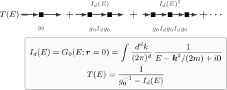
The calculation is also a perfect preview of loop diagrams. Repeated scattering from the fixed contact potential gives a geometric resolvent series. The divergent object is the free Green function evaluated at coincident points. In a nonrelativistic field theory the same algebra becomes a bubble sum after the loop energy is integrated out. Renormalization means replacing the singular bare strength g0 by a measurable low-energy parameter such as a scattering length or a binding energy. The derivation keeps three objects distinct: the cutoff-dependent bare coupling g0(Λ), the coincident-point Green function Id(E,Λ), and cutoff-independent observables such as pole positions, the three-dimensional scattering length a, or the two-dimensional binding energy B2.
Resolvent and scattering normalization. We use d for the number of spatial dimensions. The nonrelativistic Hamiltonian is
H=H0+V,H0=2mp2,
and momentum states obey
⟨k∣k′⟩=(2π)dδ(d)(k−k′).
For positive energy,
E=2mp2,p>0,
we define the outgoing free resolvent by
G0(E;k)=E−k2/(2m)+i01.
The T matrix is defined by the Lippmann–Schwinger equation T=V+VG0T. Overall signs in the scattering amplitude differ across books because some define f with an extra minus sign relative to T. The pole locations, cutoff dependence, and low-energy denominators below are convention-independent.
The exact scattering state with incoming momentum p satisfies
Repeated scattering from a contact interaction gives a geometric series. The whole ultraviolet problem is contained in the coincident Green function Id(E)=G0(E;r=0).
In coordinate space the same object is even more transparent. Since
V(r)=g0δ(d)(r),
the scattering wavefunction has the form
ψp(+)(r)=eip⋅r+g0G0(E;r)ψp(+)(0),
where
G0(E;r)=∫Λ(2π)dddkE−k2/(2m)+i0eik⋅r.
Setting r=0 gives
ψp(+)(0)=1+g0G0(E;0)ψp(+)(0),
so the same denominator appears. The singularity of the zero-range potential is the singularity of the free Green function at coincident points.
The measure contributes kd−1dk, so the high-momentum behavior is
Id∼−2m∫Λdkkd−3.
Therefore:
spatial dimensiond=1d=2d=3d>3UV behavior of IdfinitelogΛΛΛd−2meaninga delta potential is a genuine potentiala scale is generated by renormalizationthe bare coupling must be tunedmore short-distance data are needed
This is the quantum-mechanical version of power counting. The contact interaction is more singular in higher dimension because the wavefunction has more angular phase space available near the origin.
There is also a useful relation to the relativistic propagator. A scalar Feynman propagator is
Grel(p)=p02−p2−m2+i0i.
Near the positive-energy mass shell, write p0=m+E with E≪m. Then
p02−p2−m2=(m+E)2−p2−m2≃2m(E−2mp2),
so
Grel(p)≃2miE−p2/(2m)+i01.
The nonrelativistic resolvent is the positive-energy, low-velocity limit of the relativistic propagator, up to the conventional normalization factor 2m.
A finite bare coupling cannot survive the limit Λ→∞. Instead define a renormalized coupling at a subtraction scale μ by
gR(μ)1=g0(Λ)1+2πmlogμ2Λ2.
After taking the zero-range limit at fixed gR(μ),
T2(p)1=gR(μ)1+2πm[logp2μ2+iπ].
The physical amplitude cannot depend on the arbitrary scale μ. Therefore gR(μ) must run. Differentiating the definition at fixed bare coupling gives
μdμdgR(μ)1=−πm.
Equivalently,
μdμdgR=πmgR2.
This is the first beta function in the course. It is not yet a relativistic QFT beta function, but the mechanism is the same: logarithmic UV sensitivity is traded for scale dependence of a coupling.
A more physical parametrization uses the positive binding-energy magnitude. For an attractive interaction, the pole condition at p=iκ defines
B2=2mκ2>0,Ebound=−B2.
Analytic continuation gives
gR(μ)1+2πmlogκ2μ2=0.
Eliminating gR(μ) yields
T2(E)=log(B2/E)+iπ2π/m
for E>0. More generally, away from the positive-energy cut the denominator is log[B2/(−E)]; its upper-edge value is log(B2/E)+iπ. Every attractive two-dimensional zero-range interaction therefore carries one bound-state scale. The essential fact is that the dimensionless coupling mg0 has produced the energy scale B2: dimensional transmutation in its simplest nonrelativistic form.
Three spatial dimensions: scattering length and resonance
For 0<p<Λ, the principal value and the outgoing boundary prescription give
I3(E,Λ)=π2m[−Λ+2plogΛ−pΛ+p]−2πimp.
Thus, for p≪Λ,
I3(E,Λ)=−π2mΛ−2πimp+O(Λmp2).
Thus
T3(p)1=g0(Λ)1+π2mΛ+2πimp+O(Λmp2).
The linear divergence is absorbed by defining the physical scattering length a through
g0(Λ)1+π2mΛ=2πam.
At finite sharp cutoff the matched T matrix is exactly
T3,Λ(p)=a−1+ip−δΛ(p)2π/m,δΛ(p)=πplogΛ−pΛ+p.
The cutoff correction belongs in the inverse amplitude:
T3,Λ(p)1=2πm[a−1+ip−πΛ2p2+O(Λ3p4)].
The zero-range limit at fixed a and p is therefore
T3(p)=a−1+ip2π/m.
An expansion of T3,Λ relative to this limit additionally requires
∣δΛ(p)∣≪∣a−1+ip∣. This condition must be reconsidered on
analytic continuation near a pole; an additive O(p2/Λ) error on T
would have neither the correct dimensions nor a uniform pole estimate.
The corresponding zero-range s-wave scattering amplitude is
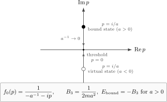
f0(p)=−2πmT3(p)=−a−1+ip1=−a−1−ip1,
and the total low-energy cross-section is
σ(p)=4π∣f0(p)∣2=a−2+p24π.
The special point a−1=0 is a zero-energy resonance, often called the unitary limit. At that point
f0(p)=pi,σ(p)=p24π,
which saturates the s-wave unitarity bound.
In the zero-range limit, the three-dimensional contact amplitude is governed by the denominator a−1+ip. For a>0 the pole at p=i/a is a bound state; for a<0 it is a virtual state. The resonance limit ∣a∣→∞ places the pole at threshold.
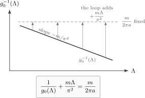
Keeping a finite while Λ changes requires a cutoff-dependent bare coupling,
g0(Λ)=−mΛ/π2+m/(2πa)1.
For large Λ,
g0(Λ)=−mΛπ2[1+2aΛπ+O((aΛ)21)].
The bare coupling goes to zero, but it goes to zero in a very specific way. A finite physical scattering length is obtained only by tuning g0(Λ) close to the cutoff-dependent critical curve.
In three dimensions, fixed physical scattering length means g0−1(Λ)+mΛ/π2=m/(2πa). Changing the cutoff changes the bare parameter while preserving a. At nonzero momentum the finite sharp cutoff leaves the inverse-amplitude correction δΛ(p); the matched amplitude approaches its zero-range limit as the cutoff grows.
This is the key renormalization lesson. A divergent bare expression can still define finite physics if the bare parameters are regarded as cutoff-dependent coordinates on a space of effective theories.
The tuning becomes especially transparent at the resonance a−1=0:
g0,c(Λ)=−mΛπ2.
A large but finite scattering length means that g0(Λ) is close to this cutoff-dependent critical curve. In other words, the low-energy resonance is not produced by a large bare coupling; it is produced by a precise cancellation in g0−1−I3(0,Λ).
From a singular potential to an effective field theory
A point interaction in three dimensions is not a normal function-valued potential. It is better understood as a boundary condition or as the leading term of a low-energy effective theory.
A finite-range potential of range R has an s-wave amplitude that can be expanded at low momentum as
f0(p)=−a−1+21rep2−ip+O(p4R3)1,
where a is the scattering length and re is the effective range. The zero-range contact limit captures a and has re=0; the finite sharp-cutoff approximation above instead has the regulator contribution re=4/(πΛ). A more accurate effective interaction includes derivative terms,
Veff(p′,p)=C0(Λ)+C2(Λ)(p2+p′2)+C4(Λ)(p4+⋯)+⋯.
The scattering-length sign, effective-range expansion and equal-mass Born
normalization are given in
Braaten and Hammer 2006, § 2.1, pp. 11–13, PDF.
Their m is the constituent mass M in the translation above; the sharp-cutoff
correction displayed here follows from our explicit principal-value integral.
The coefficients C0,C2,… are not determined by the zero-range idealization. They must be matched to physical low-energy data: scattering length, effective range, and higher threshold parameters. This is the nonrelativistic version of the Wilsonian operator expansion.
The same structure appears in a nonrelativistic field theory with constituent
mass M and Lagrangian
L=ψ†(i∂t+2M∇2)ψ−2C0(ψ†ψ)2+2C2[∇(ψ†ψ)]2+⋯.
The quartic vertex C0 generates the same geometric bubble structure as the
potential problem. For two equal constituent masses M, the relative kinetic
denominator after the loop energy integral is E−k2/M+i0. Thus the spatial
resolvent is Id with its fixed-center mass replaced by M/2; the vertex and external-state
normalizations must also be matched. The contact potential supplies a simple
exact example of a local interaction whose repeated short-distance
fluctuations require renormalization.
In three dimensions, elastic unitarity for a single s-wave channel implies
Imf0(p)1=−p(p>0).
The zero-range contact result gives
f0(p)=−a−1−ip1,
so
f0(p)1=−a−1−ip.
Therefore
Imf0(p)1=−p,
exactly as required. The real part −a−1 is dynamical data. The imaginary part −p is fixed by open phase space and probability conservation. This is why the low-energy denominator a−1+ip is more robust than any particular cutoff calculation.
Relativistic preview: a small coupling and a large logarithm
The manuscript next applies the same lesson to four-dimensional ϕ4 theory. A one-loop correction to the four-point vertex contains the schematic Euclidean integral
up to channel-dependent combinatorial coefficients and local terms. The perturbative parameter is therefore not just λ0, but
16π2λ0logq2Λ2.
When this combination becomes order one, terms with the highest power of the logarithm at each loop order must be resummed even if λ0 is small. The next lessons develop the scalar loop integral, the one-loop four-point function, leading logarithms, and the renormalization-group equation in detail.
A contact interaction is the smallest model in which renormalization is unavoidable but completely explicit.
In one spatial dimension, G0(E;0) is finite and the delta-function potential is an ordinary exactly solvable interaction. In two dimensions, the coincident Green function diverges logarithmically, producing a running coupling and a dynamically generated scale. In three dimensions, the divergence is linear; the bare coupling must be tuned with the cutoff so that the physical scattering length remains fixed.
The exact contact amplitude is a geometric series,
T(E)=g0−1−Id(E,Λ)1.
The integral Id is the coincident nonrelativistic resolvent; after replacing
its kinetic mass by the reduced mass, the same spatial integral appears in
the two-body bubble. The renormalized answer is obtained by replacing the
unobservable bare coefficient g0(Λ) by physical low-energy data such
as a or B2.
The three-dimensional zero-range result
T3(p)=a−1+ip2π/m
is the prototype for much of what follows: a short-distance singularity is absorbed into a local parameter, while the remaining energy dependence is fixed by long-distance propagation and unitarity.
Treating g0 as an observable. The bare strength of a point interaction depends on the cutoff and regulator. The observable is the scattering amplitude, or equivalently low-energy parameters such as a and re.
Confusing the cutoff with the physical range. A cutoff Λ is a calculation device. A real finite-range potential has a physical range R. A sensible EFT calculation takes p≪Λ while matching coefficients to physics at scales of order R−1.
Dropping the i0. The imaginary part of Id is not a detail. It fixes outgoing boundary conditions and enforces elastic unitarity.
Expecting the same behavior in all dimensions. The contact interaction is finite in d=1, logarithmic in d=2, and linearly divergent in d=3. Dimensionality changes the physics.
Calling every divergence a failure. The divergence tells us that the zero-range interaction needs a matching condition. Once matched, it makes finite low-energy predictions.
More precisely, expanding the logarithm in the exact principal value gives
T3,Λ(p)1=2πm[a−1+ip−πΛ2p2+O(Λ3p4)].
Taking Λ→∞ at fixed a,p gives
T3(p)=(2π/m)/(a−1+ip). Inverting the expansion at finite cutoff
requires the denominator correction to be small compared with
a−1+ip; it is not a uniform approximation near a continued pole.
Braaten, Eric, and Hans-Werner Hammer. “Universality in Few-Body Systems with Large Scattering Length.” Physics Reports428 (2006): 259–390. DOI. Open PDF, version 3, 18 August 2006; locators above use the printed preprint pages.
Hammer, Hans-Werner, and Richard J. Furnstahl. “Effective Field Theory for Dilute Fermi Systems.” Nuclear Physics A678, nos. 3–4 (2000): 277–294.
Kaplan, David B., Martin J. Savage, and Mark B. Wise. “A New Expansion for Nucleon–Nucleon Interactions.” Physics Letters B424, nos. 3–4 (1998): 390–396.
Schwartz, Matthew D. Quantum Field Theory and the Standard Model. Cambridge: Cambridge University Press, 2014, Chapters 22–23.
Srednicki, Mark. Quantum Field Theory. Cambridge: Cambridge University Press, 2007, Sections 27–29.
Weinberg, Steven. The Quantum Theory of Fields. Volume I: Foundations. Cambridge: Cambridge University Press, 1995, Chapter 3.
Zee, A. Quantum Field Theory in a Nutshell. 2nd ed. Princeton: Princeton University Press, 2010.
Original QFT.org content:CC BY 4.0, unless an item supplies different terms. Third-party material retains its own terms.