

Interaction Picture and Dyson Expansion
The previous pages built free relativistic fields as collections of harmonic oscillators. That construction is powerful because the free theory is exactly solvable: one knows its energy eigenstates, its mode expansion, and eventually its propagators. But the physics we actually want is not free. Interactions scatter particles, shift masses, mix states, and create correlations between field operators at different spacetime points.
The first problem of perturbative QFT is therefore not to draw diagrams. It is to write the exact time evolution in a form that separates the part we can solve from the part we will expand in. The interaction picture does precisely that. The free Hamiltonian is used to evolve operators, while the interaction evolves states. The result is the Dyson expansion, a time-ordered exponential that is the operator ancestor of Feynman diagrams.
For a complementary treatment that emphasizes ordered integration domains, switching, regulators, and the limits imposed by Haag’s theorem, see The Interaction Picture and Dyson Series.
Splitting the Hamiltonian
Section titled “Splitting the Hamiltonian”In the Schrödinger picture, states evolve and operators are time-independent unless they have explicit time dependence:
If , this equation is solved by
The idea of the interaction picture is to remove this known free evolution from the state:
At the same time, every Schrödinger-picture operator is converted into a free-evolving interaction-picture operator
Thus the interaction picture is halfway between the Schrödinger and Heisenberg pictures. In the Schrödinger picture, all dynamics is carried by the state. In the Heisenberg picture, all dynamics is carried by operators. In the interaction picture, the exactly solvable free dynamics is carried by operators, while the remaining interaction dynamics is carried by the state.
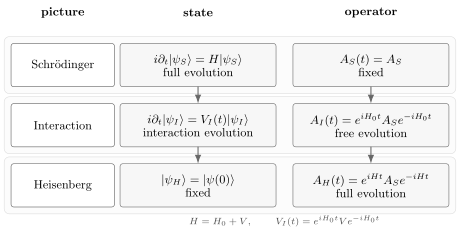
The interaction picture splits the dynamics. Operators evolve with , while states evolve with the interaction Hamiltonian . This is the natural framework for perturbation theory because the free theory supplies known oscillators, states, and propagators.
Different pictures are not different theories. They are different ways of distributing the same unitary time evolution between states and operators. The interaction picture is useful because it makes the perturbative small parameter appear in the equation of motion.
The interaction-picture equation
Section titled “The interaction-picture equation”Differentiate the interaction-picture state:
Using the Schrödinger equation,
we obtain
Therefore
where
This equation looks like the Schrödinger equation, but with two important differences. First, the Hamiltonian on the right is only the interaction, not the full Hamiltonian. Second, even if has no explicit time dependence in the Schrödinger picture, usually has time dependence because it is conjugated by .
For example, if are eigenstates of with energies , then matrix elements of the interaction-picture interaction are
The phases are the free oscillations. Perturbation theory is built by integrating these oscillations against interaction matrix elements.
The evolution operator
Section titled “The evolution operator”Define by
Then obeys
It also satisfies the composition rule
and, since is Hermitian when is Hermitian, it is unitary:
Let denote full Schrödinger-picture evolution. With the same fixed reference time at both endpoints,
For time-independent , this becomes
The two endpoint factors are essential: in a product of adjacent propagators, , so Schrödinger-picture composition immediately gives the displayed interaction-picture composition law. The definition and evolution equation appear in Weinberg 1995, § 3.5, pp. 142–143.
If , the formula reduces to . One may choose any other fixed reference time for all states, operators, and intervals, but resetting it separately at every lower endpoint changes the picture between factors. The expression , used with a newly chosen reference for each segment, generally does not satisfy the stated composition law when .
The equation for can be written as an integral equation:
This form is the starting point of Dyson’s expansion. Iterating once gives
After iterations,
The nested limits enforce
This ordering is not cosmetic. Operators at different times need not commute:
So the product is genuinely different from .
Time ordering
Section titled “Time ordering”For two bosonic operators, time ordering means
where is the step function. For three operators, sums over all six possible time orderings. For example, the term for is
In general, places the operator with the latest time at the far left, the next latest time next, and so on. For fermionic fields, each exchange of fermionic operators introduces a minus sign; the bosonic definition above is enough for the present page, but the sign matters later for Dirac fields.
The nested second-order integral can be rewritten over the full square :
The factor compensates for the two equivalent triangular regions. At order , the same reasoning gives a factor because the -dimensional cube is divided into ordered simplices.
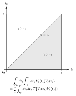
The second-order term first appears as an integral over the ordered region . Time ordering lets us integrate over the full square and divide by . At order , the same geometry replaces one ordered simplex by the full -cube divided by .
Therefore the Dyson series becomes
This is abbreviated as the time-ordered exponential
The notation means the series above. It is not the ordinary exponential unless all the commute with one another.
Combining this with the full evolution operator gives
This is one of the central identities of perturbative quantum field theory.
Ordered insertions as perturbation theory
Section titled “Ordered insertions as perturbation theory”The expansion has a simple picture. The system evolves freely except at a sequence of interaction insertions. If the insertions occur at times , the latest insertion is written on the left because operators act on states from right to left.
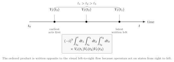
A term in the Dyson expansion is a free history interrupted by interaction insertions. The ordered region contributes the product . The symbol performs the corresponding ordering automatically for all regions of integration.
This is already the skeleton of Feynman perturbation theory. In a field theory, is typically an integral of an interaction Hamiltonian density,
Then the Dyson expansion contains spacetime integrals of products of free fields. Wick’s theorem, introduced later, will turn those time-ordered products of free fields into propagators and diagrams.
A common example is scalar theory. When there are no derivative interactions, one often has
so if
then
The first-order term in is therefore
This is the operator origin of the familiar vertex factor in perturbation theory. The factor of comes from time evolution; the spacetime integral comes from summing over where the interaction occurs; the is the symmetry normalization of the interaction.
Why the ordinary exponential is wrong
Section titled “Why the ordinary exponential is wrong”It is tempting to write
This is generally wrong. To see why, expand the ordinary exponential to second order:
The second-order term has the same operator order throughout the square. But the correct expression must use in the region and in the region . The two are equal only if
for all times. Quantum fields do not generally satisfy this condition.
This failure is the same noncommutativity that makes the Baker–Campbell–Hausdorff formula nontrivial. The interaction picture gives a useful version of that formula. For fixed operators and , define
Then
where the parameter is ordered just like time. Expanding to first order in gives Duhamel’s formula,
This is the same mechanism as
The free Hamiltonian is treated exactly, and the interaction is conjugated into the frame that rotates with the free motion.
Transition amplitudes and energy conservation
Section titled “Transition amplitudes and energy conservation”The simplest physical use of the Dyson expansion is the first-order transition amplitude. Suppose and are eigenstates of with energies and . To first order,
Using
we get
Shifting the integration variable to contributes the overall phase , which does not change the transition probability. For a long time interval , the remaining integral is sharply peaked when :
The one-sided integral from to becomes increasingly narrow as grows, but it does not by itself converge pointwise to . In the -matrix one instead uses an integral over the whole time axis, understood with symmetric limits or adiabatic switching. Distributionally,
This is the first appearance of a central theme: conservation laws in scattering amplitudes arise from integrating interaction insertions over spacetime. In actual scattering calculations one also uses wave packets, so the delta distribution is paired with smooth external-state profiles rather than treated as an ordinary square-integrable function. These qualifications prepare the later passage from amplitudes to rates and cross sections.
Toward correlation functions
Section titled “Toward correlation functions”The Dyson expansion also explains why time-ordered products dominate perturbative QFT. If and are free-evolving operators, then an interacting matrix element can be expanded schematically as
The exponential supplies all possible interaction insertions. The time-ordering symbol places those insertions and the observed operators into a single chronological product. With adiabatic switching and the asymptotic limits understood, the Gell-Mann–Low formula for vacuum expectation values contains the normalized ratio
where is the free vacuum. The limiting prescription is essential: without it, the displayed ratio is only schematic and need not relate the free and interacting vacua. Its denominator removes vacuum bubbles disconnected from the observed operators. This cancellation will become explicit when generating functionals are introduced. In the next pages, the numerator structure becomes the time-ordered Green function
and then Wick’s theorem turns the free-theory time-ordered products into contractions. That is the bridge from the operator identity derived here to Feynman diagrams.
Summary
Section titled “Summary”The interaction picture is the correct perturbative frame for QFT. It uses the free Hamiltonian to define the simple oscillatory time dependence of fields and uses the interaction to evolve states. In regulated finite systems this split is exact; in continuum QFT it is the controlled formal starting point for perturbative expansions. The approximation enters when the interaction-picture evolution operator is expanded in powers of and truncated.
The central result is Dyson’s formula,
The time-ordering symbol is essential because interaction-picture operators at different times need not commute. Its expansion converts nested ordered integrals into full time integrals with a factor . In field theory, those ordered products become the raw material for Wick contractions, propagators, vertices, and eventually scattering amplitudes.
Physically, perturbation theory describes free propagation interrupted by interaction events at all possible times. The Dyson expansion sums over the number, location, and chronological ordering of those events.
Common pitfalls
Section titled “Common pitfalls”-
Dropping time ordering. The formula is valid only when for all times. In QFT this is not generally true.
-
Confusing with . The interaction-picture interaction is not usually time-independent. It is , so it carries free-theory phases.
-
Putting the earliest operator on the left. Time ordering places the latest time on the left. This agrees with the fact that operators act on states from right to left.
-
Forgetting fermion signs. For bosonic operators, time ordering just reorders the operators. For fermionic fields, each exchange of fermionic operators contributes a minus sign.
-
Assuming always. This relation is common for non-derivative interactions, but derivative interactions and constrained systems require more care.
Exercises
Section titled “Exercises”Exercise 1: deriving the interaction-picture equation
Section titled “Exercise 1: deriving the interaction-picture equation”Let
Derive the interaction-picture Schrödinger equation
Solution
Differentiate:
The Schrödinger-picture state obeys
so
Substitute this into the derivative of :
Therefore
with
Exercise 2: from ordered triangles to time ordering
Section titled “Exercise 2: from ordered triangles to time ordering”Show that
Solution
The full square of integration is the union of two triangular regions:
The diagonal has measure zero and does not affect the integral. By definition,
Thus
In the second integral, exchange the dummy labels . It becomes another copy of the first integral. Therefore the full square integral is twice the ordered triangular integral, giving the desired factor .
Exercise 3: first-order transition amplitude
Section titled “Exercise 3: first-order transition amplitude”Let . Compute the first-order transition amplitude from to over the time interval .
Solution
At first order,
For ,
Since
we have
Therefore
If , then
For large , the magnitude is sharply peaked near . The one-sided finite-time integral itself should not be identified with a delta function. In scattering theory the energy-conserving delta distribution comes from the whole time axis with an adiabatic regulator:
Exercise 4: when time ordering becomes unnecessary
Section titled “Exercise 4: when time ordering becomes unnecessary”Assume for all . Show that the Dyson expansion reduces to the ordinary exponential.
Solution
If all the commute, time ordering no longer changes any product:
The Dyson series becomes
This is exactly the Taylor series of the ordinary exponential:
Thus time ordering is needed precisely because the interaction-picture interactions generally fail to commute at different times.
References and further reading
Section titled “References and further reading”- Sidney Coleman, Lectures on Quantum Field Theory, Chapter 7, especially the interaction picture and Dyson’s formula.
- Mark Srednicki, Quantum Field Theory, Sections 6–9, for the connection between time evolution, perturbation theory, and path integrals.
- Weinberg, Steven. The Quantum Theory of Fields, Volume I: Foundations. Cambridge: Cambridge University Press, 1995. First edition; 2005 paperback, seventh printing 2012 consulted. § 3.5, pp. 142–143 supports the interaction-picture evolution used here; § 6.1 is further reading. DOI.
- A. Zee, Quantum Field Theory in a Nutshell, Chapters I.7–I.9, for a compact physical introduction to Feynman diagrams and perturbing the vacuum.
Original QFT.org content:CC BY 4.0, unless an item supplies different terms. Third-party material retains its own terms.