Statistics, Occupation Algebra, and Anyons

The field operators introduced so far were bosonic: their creation operators commute, so multiparticle wavefunctions are symmetric. That is not a small technical choice. The sign or phase acquired when identical particles are exchanged is part of the quantum definition of the particles.

For bosons, arbitrarily many quanta may occupy the same one-particle state. For fermions, the algebra itself enforces the Pauli exclusion principle: a single mode has only two states, empty and occupied. In the plane, particle worldlines can braid around each other, and an exchange may carry a phase $e^{i\theta}$ that is neither $+1$ nor $-1$. This is abelian anyon statistics.

The aim of this page is to connect exchange symmetry of wavefunctions, occupation algebra, and the topology of particle paths. The exchange argument fixes $N\geq2$ identical point particles in Euclidean $\mathbb R^d$, excludes collisions, and first considers scalar exchange sectors, in which each exchange acts by a phase. This nonrelativistic argument does not derive the relativistic spin–statistics theorem. Under its assumptions on local relativistic fields, that theorem connects integer spin to Bose statistics and half-integer spin to Fermi statistics; its treatment belongs to the later Dirac-field and Lorentz-group lessons. See Srednicki 2006, § 4, pp. 45–48 (author manuscript, PDF).

Exchange symmetry and operator algebra

For two identical particles, the labels $1$ and $2$ are bookkeeping devices, not physical labels. If a two-particle wavefunction is written as $\rho(x_1,x_2)$, then exchanging the arguments must give an equivalent state. In the scalar exchange sectors considered here, the two possibilities in three-dimensional Euclidean space are

$$\rho(x_1,x_2)=+\rho(x_2,x_1)$$

for bosons and

$$\rho(x_1,x_2)=-\rho(x_2,x_1)$$

for fermions. More generally, for $N$ identical particles, a permutation $\tau\in S_N$ acts by

$$\rho(x_{\tau(1)},x_{\tau(2)},\ldots,x_{\tau(N)}) =\chi(\tau)\rho(x_1,x_2,\ldots,x_N).$$

For bosons, $\chi(\tau)=1$. For fermions,

$$\chi(\tau)=\operatorname{sgn}(\tau).$$

In the operator language, these two choices become two different algebras. A bosonic mode is created and destroyed by $a_i^\dagger$ and $a_i$ with

$$[a_i,a_j^\dagger]=\delta_{ij}, \qquad [a_i,a_j]=0, \qquad [a_i^\dagger,a_j^\dagger]=0.$$

A fermionic mode is created and destroyed by $c_i^\dagger$ and $c_i$ with

$$\{c_i,c_j^\dagger\}=\delta_{ij}, \qquad \{c_i,c_j\}=0, \qquad \{c_i^\dagger,c_j^\dagger\}=0.$$

Here

$$[A,B]=AB-BA, \qquad \{A,B\}=AB+BA.$$

The commutator says that two bosonic creation operators may pass through each other without changing the state. The anticommutator says that two fermionic creation operators pick up a minus sign when interchanged:

$$c_i^\dagger c_j^\dagger=-c_j^\dagger c_i^\dagger.$$

This is why the algebra is more fundamental than the notation. Once the algebra is chosen, the symmetry or antisymmetry of all multiparticle states follows automatically.

Bosonic occupation numbers

For one bosonic oscillator, the algebra is

$$[a,a^\dagger]=1.$$

Let $|0\rangle$ be the normalized vacuum of this mode,

$$a|0\rangle=0, \qquad \langle0|0\rangle=1.$$

The normalized $n$-particle state is

$$|n\rangle=\frac{1}{\sqrt{n!}}(a^\dagger)^n|0\rangle.$$

The ladder operators act as

$$a^\dagger|n\rangle=\sqrt{n+1}\,|n+1\rangle, \qquad a|n\rangle=\sqrt n\,|n-1\rangle.$$

The number operator

$$N=a^\dagger a$$

satisfies

$$N|n\rangle=n|n\rangle.$$

The square roots are not arbitrary normalization decorations. They are forced by the commutation relation. For example,

$$\begin{aligned} a^\dagger|n\rangle &=\frac{1}{\sqrt{n!}}(a^\dagger)^{n+1}|0\rangle \\ &=\sqrt{n+1}\,\frac{1}{\sqrt{(n+1)!}}(a^\dagger)^{n+1}|0\rangle \\ &=\sqrt{n+1}\,|n+1\rangle. \end{aligned}$$

Similarly,

$$a(a^\dagger)^n=(a^\dagger)^n a+n(a^\dagger)^{n-1},$$

so

$$a|n\rangle=\sqrt n\,|n-1\rangle.$$

Bosonic occupation is unbounded:

$$n=0,1,2,3,\ldots.$$

This unbounded ladder permits macroscopic occupation of a single mode. For $n\gg1$, the adjacent ladder coefficients satisfy $\sqrt{n+1}/\sqrt n=1+O(n^{-1})$, but this does not by itself justify replacing the operators by a classical amplitude. In a number state, orthogonality gives $\langle n|a|n\rangle=0$, whereas $\langle n|a^\dagger a|n\rangle=n$; no single complex amplitude reproduces both moments. A classical field approximation needs additional assumptions about the state and its fluctuations, as explained in the coherent and selected-phase descriptions of the preceding lesson.

The fermionic oscillator

For one fermionic mode, the algebra is

$$\{c,c^\dagger\}=1, \qquad \{c,c\}=0, \qquad \{c^\dagger,c^\dagger\}=0.$$

The last two equations imply

$$c^2=0, \qquad (c^\dagger)^2=0.$$

With a normalized vacuum

$$c|0\rangle=0,$$

there is only one nonzero excited state,

$$|1\rangle=c^\dagger|0\rangle.$$

Trying to create a second particle in the same mode gives

$$c^\dagger|1\rangle=(c^\dagger)^2|0\rangle=0.$$

This is the Pauli exclusion principle in its most economical form. It is not added after quantization; it is contained in the algebra.

The annihilation operator obeys

$$c|1\rangle=cc^\dagger|0\rangle=(1-c^\dagger c)|0\rangle=|0\rangle.$$

The number operator

$$N=c^\dagger c$$

has eigenvalues only $0$ and $1$:

$$N|0\rangle=0, \qquad N|1\rangle=|1\rangle.$$

One also finds

$$N^2=N.$$

Thus $N$ is a projection operator. A fermionic mode is either empty or occupied; there is no intermediate occupation number and no double occupation.

In the ordered basis $(|0\rangle,|1\rangle)$, one convenient matrix representation is

$$c= \begin{pmatrix} 0&1\\ 0&0 \end{pmatrix}, \qquad c^\dagger= \begin{pmatrix} 0&0\\ 1&0 \end{pmatrix}, \qquad N= \begin{pmatrix} 0&0\\ 0&1 \end{pmatrix}.$$

These matrices obey $\{c,c^\dagger\}=1$ and $(c^\dagger)^2=0$ exactly.

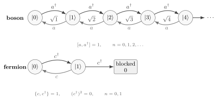
A bosonic mode has an infinite occupation-number ladder, with $a^\dagger|n\rangle=\sqrt{n+1}|n+1\rangle$. A fermionic mode has only two states: $|0\rangle$ and $|1\rangle=c^\dagger|0\rangle$. The algebra $(c^\dagger)^2=0$ blocks the next rung.

Many fermionic modes

For many fermionic modes, the anticommutation relations are

$$\{c_p,c_q^\dagger\}=\delta_{pq}, \qquad \{c_p,c_q\}=0, \qquad \{c_p^\dagger,c_q^\dagger\}=0.$$

Here $p,q$ may be discrete labels, such as momenta in a finite box. An ordered $N$-fermion state is

$$|p_1,p_2,\ldots,p_N\rangle =c_{p_1}^\dagger c_{p_2}^\dagger\cdots c_{p_N}^\dagger|0\rangle.$$

Interchanging two creation operators changes the sign:

$$|p_2,p_1,p_3,\ldots,p_N\rangle =-|p_1,p_2,p_3,\ldots,p_N\rangle.$$

If two labels coincide, the state vanishes. For example,

$$c_p^\dagger c_p^\dagger|0\rangle=0.$$

The annihilation operator removes a matching particle and produces a sign determined by how many fermionic operators it must pass. Acting on an ordered state,

$$c_q|p_1,p_2,\ldots,p_N\rangle = \sum_{r=1}^{N}(-1)^{r-1}\delta_{q p_r} |p_1,\ldots,\widehat{p_r},\ldots,p_N\rangle.$$

The hat means that the entry is omitted. For instance,

$$c_q|p_1,p_2,p_3\rangle =\delta_{q p_1}|p_2,p_3\rangle -\delta_{q p_2}|p_1,p_3\rangle +\delta_{q p_3}|p_1,p_2\rangle.$$

This formula is the many-mode form of Pauli exclusion and antisymmetry. It is also the first place where fermionic signs become unavoidable in calculations. Later, the same bookkeeping will appear as the minus signs attached to fermion exchanges and closed fermion loops in Feynman diagrams.

The fermionic number operator for mode $p$ is

$$N_p=c_p^\dagger c_p,$$

and the total number operator is

$$N=\sum_p c_p^\dagger c_p.$$

Each $N_p$ has eigenvalues $0$ and $1$. The total particle number is still an integer, but it is now a sum of binary occupation numbers.

A q-oscillator toy model

A useful algebraic toy model interpolates between the bosonic and fermionic ladder formulas:

$$aa^\dagger-q a^\dagger a=1.$$

For the Hilbert-space derivation, first take $q$ to be real and let $a^\dagger$ be the Hermitian adjoint of $a$. Then squared ladder coefficients must be real and nonnegative. The complex root-of-unity continuation considered below is a formal algebraic observation, not a positive-norm Fock representation of this same $*$-algebra.

Assume a vacuum

$$a|0\rangle=0,$$

and define normalized states so that

$$a^\dagger|n\rangle=\alpha_n|n+1\rangle, \qquad a|n+1\rangle=\alpha_n^*|n\rangle.$$

Let

$$\gamma_n=|\alpha_n|^2.$$

Then

$$aa^\dagger|n\rangle=\gamma_n|n\rangle, \qquad a^\dagger a|n\rangle=\gamma_{n-1}|n\rangle,$$

where $\gamma_{-1}=0$ because $a|0\rangle=0$. Acting with the deformed algebra on $|n\rangle$ gives

$$\gamma_n-q\gamma_{n-1}=1.$$

Therefore

$$\gamma_0=1, \qquad \gamma_1=1+q, \qquad \gamma_2=1+q+q^2,$$

and in general

$$\boxed{\gamma_n=1+q+q^2+\cdots+q^n =\frac{1-q^{n+1}}{1-q}}$$

when $q\ne1$. It is common to write this as a $q$-number,

$$\gamma_n=[n+1]_q.$$

For real $q>-1$, all these coefficients are positive and the ladder is infinite. At $q=-1$ the first attempted second-occupation coefficient vanishes. For $q<-1$, already $\gamma_1=1+q<0$, so the assumed positive-norm representation fails.

The two familiar cases are recovered immediately.

For $q=1$,

$$\gamma_n=n+1,$$

so

$$a^\dagger|n\rangle=\sqrt{n+1}\,|n+1\rangle.$$

This is the ordinary bosonic oscillator.

For $q=-1$,

$$\gamma_0=1, \qquad \gamma_1=1+(-1)=0.$$

Thus

$$a^\dagger|0\rangle=|1\rangle, \qquad a^\dagger|1\rangle=0.$$

The ladder truncates after one particle, as in the fermionic oscillator. This reproduces the occupation rule of a single fermionic mode; it does not by itself impose anticommutation relations between distinct modes.

A particularly suggestive choice is

$$q=e^{2\pi i/N}.$$

For $N>2$ this $q$ is complex. Formally continuing the polynomial $q$-number gives

$$[N]_q=1+q+\cdots+q^{N-1}=0.$$

At the level of the formal recurrence, this would terminate the ladder at $|N-1\rangle$ and resembles a generalized exclusion rule. It cannot be read as $|\alpha_{N-1}|^2=0$ while the earlier coefficients are complex: a squared norm cannot be complex.

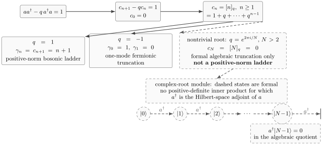
For real $q$, the deformed algebra $aa^\dagger-q a^\dagger a=1$ gives the recurrence $\gamma_n-q\gamma_{n-1}=1$, hence $\gamma_n=[n+1]_q$. The bosonic limit is $q=1$. The one-mode fermionic occupation rule appears at $q=-1$. A nonreal root of unity gives only a formal truncated recurrence, not a realization of this relation with the creation symbol identified as the involutive adjoint.

This calculation is pedagogically useful, but it needs a warning. The algebra above is not, by itself, the full physical theory of anyons. Indeed, taking the adjoint of

$$aa^\dagger-q a^\dagger a=1$$

replaces $q$ by $q^*$. If both equations are to hold with the ordinary adjoint on a nontrivial positive Hilbert space, $q$ must be real. For nonreal $q$, a construction must modify this relation or the identification of the creation symbol with the involutive adjoint; an indefinite inner product alone cannot make the stated algebra consistent. Indeed, subtracting the adjoint relation gives $a^\dagger a=0$, hence $aa^\dagger=1$; associativity then gives $a^\dagger=a^\dagger(aa^\dagger)=(a^\dagger a)a^\dagger=0$, contradicting $aa^\dagger=1$. This argument does not use positivity; for unbounded operators, assume a nonzero common invariant domain on which these products and relations hold. Even when a root of unity produces a formal exclusion rule, that rule is not the same thing as a braid-group exchange phase. Genuine anyonic statistics is best understood from the topology of particle exchange in two spatial dimensions, not merely from replacing a commutator by a $q$-commutator.

Anyons and braid statistics

Fix $N\geq2$ identical point particles in Euclidean $\mathbb R^d$ with distinct positions. The ordered configuration space is $F_N(\mathbb R^d)=(\mathbb R^d)^N\setminus\Delta$, where $\Delta$ is the set on which at least two positions coincide. Identifying configurations related by a permutation gives the unordered space $C_N(\mathbb R^d)=F_N(\mathbb R^d)/S_N$. An exchange history is a loop in this unordered space. Its class records which deformations into other exchange histories are possible without collisions. Loop classes compose to form the fundamental group; a scalar exchange sector assigns each class a phase through a one-dimensional unitary representation.

For $d\geq3$, the ordered space $F_N(\mathbb R^d)$ is simply connected: every loop of labeled configurations can be contracted without collisions. The geometric reason is that a contraction sweeps a two-dimensional disk, whereas each coincidence condition imposes $d$ independent constraints; for $d>2$ the disk can be displaced to avoid all coincidence sets. Now lift an unordered exchange loop by following labels along the paths. Its final labels differ from the initial ones by a permutation. Every permutation can occur, and histories with the same final permutation differ by a contractible loop in the ordered space. Thus the unordered loop classes are exactly $S_N$. This is the configuration-space argument of Laidlaw and DeWitt 1971, pp. 1377–1378 (PDF).

The elementary transposition $\sigma_i$, which swaps labels $i$ and $i+1$, therefore obeys

$$\sigma_i^2=1.$$

A one-dimensional unitary representation therefore sends

$$\sigma_i\mapsto \eta, \qquad \eta^2=1,$$

so

$$\eta=+1 \qquad\text{or}\qquad \eta=-1.$$

All transpositions are conjugate in $S_N$, so a scalar representation assigns them the same sign. The two choices give Bose and Fermi statistics. This conclusion concerns one-dimensional unitary representations; the permutation group also has higher-dimensional representations, which this calculation does not exclude.

In the plane, a pair of particles has a nonzero relative position in $\mathbb R^2\setminus\{0\}$. A full winding of that relative position around the origin cannot contract without a collision. This already distinguishes a double exchange from doing nothing. With fixed particle number, the worldlines progress forward in time and form braids: their deformation classes give $\pi_1(C_N(\mathbb R^2))=B_N$. The elementary braid $\sigma_i$ and its inverse describe opposite orientations of exchange. Its generators obey

$$\sigma_i\sigma_{i+1}\sigma_i = \sigma_{i+1}\sigma_i\sigma_{i+1}, \qquad \sigma_i\sigma_j=\sigma_j\sigma_i\quad(|i-j|\geq2),$$

but there is no relation $\sigma_i^2=1$. These are the planar braid relations; see Nayak et al. 2008, § II.A.1, manuscript pp. 3–4, Eqs. (1)–(5) (PDF). Spaces with punctures or different global topology require their own configuration-space analysis.

For scalar phases, the first braid relation makes neighboring generators have the same phase, but puts no restriction on that common phase. A one-dimensional unitary representation may therefore assign

$$\sigma_i\mapsto e^{i\theta},$$

with arbitrary real $\theta$ modulo $2\pi$. For abelian anyons, the exchange rule for two identical particles is then

$$\rho(x_1,x_2)\longmapsto e^{i\theta}\rho(x_1,x_2)$$

for one orientation of exchange, and

$$\rho(x_1,x_2)\longmapsto e^{-i\theta}\rho(x_1,x_2)$$

for the opposite orientation. The special cases are

$$\theta=0\quad\text{bosons}, \qquad \theta=\pi\quad\text{fermions}.$$

All other values describe abelian anyons. These are statistical factors; ordinary dynamical and other path-dependent phases are separated from them. In a nonabelian exchange sector, braiding acts by unitary matrices on a degenerate state space, and some braid operations do not commute. Matrices alone are not sufficient: for example, the two-particle group $B_2\cong\mathbb Z$ has only one generator and all its operations commute. See Nayak et al. 2008, § II.A.1, manuscript pp. 3–4 (PDF). This lesson develops only the scalar exchange phases.

Follow the two paths in the schematic below upward in time. Both exchanges have the same handedness: the right-going strand passes in front at each crossing, so the particle in front changes after the first exchange. This convention defines the chosen $\sigma_i$. The endpoints return to their original positions, but the relative position has wound once.

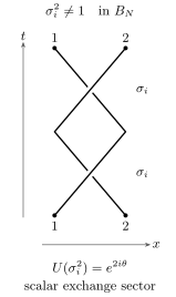
Two successive same-handed exchanges of adjacent particles in the Euclidean plane, with fixed $N\geq2$, no collisions, and any other particles held away. Time increases upward; the gaps indicate separation in the omitted transverse spatial coordinate, not collisions. The endpoints return, but $\sigma_i^2\ne1$ in $B_N$. In a scalar sector, $U(\sigma_i)=e^{i\theta}$ gives $U(\sigma_i^2)=e^{2i\theta}$; this factor can equal one, as for bosons and fermions, even though the braid remains nontrivial. For $d\geq3$, the corresponding double exchange is the identity permutation. Schematic, not to scale.

Original diagram by QFT.org, created with OpenAI Codex. Editable TikZ source · CC BY 4.0.

There is also a field-theoretic realization of this idea. In $2+1$ dimensions, coupling particles to a Chern–Simons gauge field can attach flux to charge; the integrated gauge-field constraint relates the enclosed flux to the enclosed charge. See Zee 2010, 2nd ed., § VI.1, p. 317, Eqs. (1)–(3). A full winding of one charge around another then produces an Aharonov–Bohm monodromy. For identical abelian anyons, its statistical factor is the square of the elementary exchange phase: with the orientation convention above, a full winding gives $e^{2i\theta}$ and a single exchange gives $e^{i\theta}$. This exchange-versus-winding distinction is explained in Nayak et al. 2008, § II.A.1, manuscript p. 3 (PDF).

Relation to field operators

For bosons and fermions, the field-operator version of the algebra is obtained by giving the mode label a continuous position or momentum value. At equal time,

$$[\psi_B(\mathbf x),\psi_B^\dagger(\mathbf y)] =\delta^{(d)}(\mathbf x-\mathbf y)$$

for bosons, while

$$\{\psi_F(\mathbf x),\psi_F^\dagger(\mathbf y)\} =\delta^{(d)}(\mathbf x-\mathbf y)$$

for fermions. The corresponding creation operators in momentum space obey

$$[a_{\mathbf p},a_{\mathbf q}^\dagger]=\delta_{\mathbf p\mathbf q}$$

or

$$\{c_{\mathbf p},c_{\mathbf q}^\dagger\}=\delta_{\mathbf p\mathbf q},$$

depending on the statistics.

The next step in the course is to diagonalize free nonrelativistic Hamiltonians in this language. For either bosons or fermions the free Hamiltonian takes the same formal shape,

$$H_0=\sum_{\mathbf p}\epsilon_{\mathbf p}\,A_{\mathbf p}^\dagger A_{\mathbf p}, \qquad \epsilon_{\mathbf p}=\frac{\mathbf p^2}{2m},$$

but the meaning of the occupation number differs. For bosons,

$$n_{\mathbf p}=0,1,2,\ldots,$$

while for fermions,

$$n_{\mathbf p}=0,1.$$

The same expression for $H_0$ therefore describes very different many-body physics. A Bose gas may form a condensate. A Fermi gas forms a filled Fermi sea. The distinction is not in the single-particle dispersion $\epsilon_{\mathbf p}$; it is in the occupation algebra.

Summary

The exchange statistics of identical particles is encoded algebraically by creation and annihilation operators. Bosonic operators commute, so the occupation ladder is infinite:

$$a^\dagger|n\rangle=\sqrt{n+1}\,|n+1\rangle.$$

Fermionic operators anticommute, so a single mode has only two states:

$$|0\rangle, \qquad |1\rangle=c^\dagger|0\rangle, \qquad (c^\dagger)^2=0.$$

For many fermionic modes, the sign in an annihilation formula counts how many occupied modes the annihilation operator passes through. This is the operator form of antisymmetric wavefunctions.

The deformed oscillator

$$aa^\dagger-q a^\dagger a=1$$

leads to the recurrence

$$\gamma_n-q\gamma_{n-1}=1, \qquad \gamma_n=1+q+\cdots+q^n.$$

For real $q$, it gives a compact algebraic bridge between bosonic and one-mode fermionic occupation ladders. A complex root of unity only suggests a formal generalized exclusion rule; it does not define positive norms through $\gamma_n=|\alpha_n|^2$. The exchange argument is instead topological: for fixed $N\geq2$ identical point particles in Euclidean space with collisions excluded, the group is $S_N$ for $d\geq3$ and $B_N$ in the plane. In a scalar unitary sector, the former gives only Bose/Fermi signs, while the latter permits an arbitrary exchange phase $e^{i\theta}$. The q-oscillator is a useful calculation, not a substitute for braid statistics.

The key lesson is that the same free-particle energy spectrum can lead to radically different many-body physics depending on the algebra of the creation operators. Statistics is not decoration; it is part of the definition of the quantum field.

Common pitfalls

1. Treating particle labels as physical distinctions. Artificial labels such as $1$ and $2$ can track paths in the ordered configuration space. They do not make identical particles distinct physical species or turn a label into an observable.

2. Deriving Pauli exclusion from repulsion. Pauli exclusion is not a short-range force. It follows from $(c^\dagger)^2=0$.

3. Forgetting fermionic signs or contact terms. Interchanging two creation operators, two annihilation operators, or an annihilator and a creator of distinct modes introduces a minus sign. Moving an annihilator past a creator also requires the contact term: $c_p c_q^\dagger=\delta_{pq}-c_q^\dagger c_p$.

4. Confusing the q-oscillator with physical anyons. The deformed oscillator is a useful algebraic model, but physical anyons arise from braid topology and are naturally realized in two spatial dimensions.

5. Extending the exchange argument beyond its assumptions. The planar braid group here assumes fixed particle number, Euclidean space, and no collisions. For $d\geq3$, the two scalar unitary exchange sectors give Bose and Fermi statistics; topology alone has not excluded every higher-dimensional representation or proved the relativistic spin–statistics theorem.

Exercises

Exercise 1

Verify directly that the matrices

$$c= \begin{pmatrix} 0&1\\ 0&0 \end{pmatrix}, \qquad c^\dagger= \begin{pmatrix} 0&0\\ 1&0 \end{pmatrix}$$

satisfy the one-mode fermion algebra. Compute $N=c^\dagger c$ and show that $N^2=N$.

Solution

First,

$$c^2= \begin{pmatrix} 0&1\\ 0&0 \end{pmatrix} \begin{pmatrix} 0&1\\ 0&0 \end{pmatrix} =0,$$

and similarly

$$(c^\dagger)^2=0.$$

Next,

$$cc^\dagger= \begin{pmatrix} 0&1\\ 0&0 \end{pmatrix} \begin{pmatrix} 0&0\\ 1&0 \end{pmatrix} = \begin{pmatrix} 1&0\\ 0&0 \end{pmatrix},$$

while

$$c^\dagger c= \begin{pmatrix} 0&0\\ 1&0 \end{pmatrix} \begin{pmatrix} 0&1\\ 0&0 \end{pmatrix} = \begin{pmatrix} 0&0\\ 0&1 \end{pmatrix}.$$

Therefore

$$\{c,c^\dagger\}=cc^\dagger+c^\dagger c = \begin{pmatrix} 1&0\\ 0&1 \end{pmatrix}.$$

The number operator is

$$N=c^\dagger c= \begin{pmatrix} 0&0\\ 0&1 \end{pmatrix}.$$

Thus

$$N^2= \begin{pmatrix} 0&0\\ 0&1 \end{pmatrix}^2 = \begin{pmatrix} 0&0\\ 0&1 \end{pmatrix}=N.$$

So $N$ is a projection onto the occupied state.

Exercise 2

Let

$$|p_1,p_2,p_3\rangle=c_{p_1}^\dagger c_{p_2}^\dagger c_{p_3}^\dagger|0\rangle.$$

Using the anticommutation relations, compute $c_q|p_1,p_2,p_3\rangle$.

Solution

Start from

$$c_q c_{p_1}^\dagger c_{p_2}^\dagger c_{p_3}^\dagger|0\rangle.$$

Use

$$c_q c_p^\dagger=\delta_{qp}-c_p^\dagger c_q.$$

First pass through $c_{p_1}^\dagger$:

$$c_q c_{p_1}^\dagger c_{p_2}^\dagger c_{p_3}^\dagger|0\rangle =\delta_{q p_1}c_{p_2}^\dagger c_{p_3}^\dagger|0\rangle -c_{p_1}^\dagger c_q c_{p_2}^\dagger c_{p_3}^\dagger|0\rangle.$$

Then pass through $c_{p_2}^\dagger$ in the second term:

$$-c_{p_1}^\dagger c_q c_{p_2}^\dagger c_{p_3}^\dagger|0\rangle =-\delta_{q p_2}c_{p_1}^\dagger c_{p_3}^\dagger|0\rangle +c_{p_1}^\dagger c_{p_2}^\dagger c_q c_{p_3}^\dagger|0\rangle.$$

Finally,

$$c_q c_{p_3}^\dagger|0\rangle =\delta_{q p_3}|0\rangle-c_{p_3}^\dagger c_q|0\rangle =\delta_{q p_3}|0\rangle.$$

Therefore

$$c_q|p_1,p_2,p_3\rangle =\delta_{q p_1}|p_2,p_3\rangle -\delta_{q p_2}|p_1,p_3\rangle +\delta_{q p_3}|p_1,p_2\rangle.$$

The alternating signs count how many creation operators $c_q$ passes before it annihilates the matching particle.

Exercise 3

For the deformed oscillator with real $q$,

$$aa^\dagger-q a^\dagger a=1,$$

derive

$$\gamma_n=1+q+\cdots+q^n,$$

where $a^\dagger|n\rangle=\alpha_n|n+1\rangle$ and $\gamma_n=|\alpha_n|^2$. Then evaluate the result for $q=1$ and $q=-1$.

Solution

Assume

$$a|0\rangle=0, \qquad \gamma_{-1}=0.$$

The definitions give

$$aa^\dagger|n\rangle=\gamma_n|n\rangle, \qquad a^\dagger a|n\rangle=\gamma_{n-1}|n\rangle.$$

Acting with $aa^\dagger-q a^\dagger a=1$ on $|n\rangle$ gives

$$\gamma_n-q\gamma_{n-1}=1.$$

Thus

$$\gamma_0=1,$$

and recursively

$$\gamma_1=1+q, \qquad \gamma_2=1+q+q^2,$$

so

$$\gamma_n=1+q+\cdots+q^n.$$

For $q=1$,

$$\gamma_n=n+1,$$

which gives the bosonic ladder coefficient $\sqrt{n+1}$.

For $q=-1$,

$$\gamma_0=1, \qquad \gamma_1=1-1=0.$$

Therefore $a^\dagger|1\rangle=0$, so the ladder truncates after the first occupied state, as for a fermionic mode.

Exercise 4

Fix $N\geq2$ identical point particles in Euclidean $\mathbb R^d$, exclude collisions, and work in a one-dimensional unitary exchange sector. For $d\geq3$, an elementary exchange in the permutation group satisfies $\sigma^2=1$. Show that the only possible exchange phases are $+1$ and $-1$. Then explain why the same argument fails for the braid group in the plane.

Solution

In a one-dimensional unitary representation, the exchange generator is represented by a phase:

$$\sigma\mapsto e^{i\theta}.$$

If the group relation is

$$\sigma^2=1,$$

then the representation must obey

$$e^{2i\theta}=1.$$

Therefore

$$e^{i\theta}=+1 \qquad\text{or}\qquad e^{i\theta}=-1.$$

These are Bose and Fermi statistics.

In two spatial dimensions, exchange is represented by a braid generator. The braid group does not impose $\sigma^2=1$. A double exchange is a nontrivial winding, not a path that can generally be deformed to doing nothing. Therefore a one-dimensional representation may assign

$$\sigma\mapsto e^{i\theta}$$

with arbitrary $\theta$ modulo $2\pi$. This gives abelian anyon statistics.

References

• Laidlaw, Michael G. G., and Cécile Morette DeWitt. “Feynman Functional Integrals for Systems of Indistinguishable Particles.” Physical Review D 3 (1971), 1375–1378. DOI. Open PDF.
• Nayak, Chetan, Steven H. Simon, Ady Stern, Michael Freedman, and Sankar Das Sarma. “Non-Abelian Anyons and Topological Quantum Computation.” Reviews of Modern Physics 80 (2008), 1083–1159. DOI. Open PDF, accepted manuscript, arXiv:0707.1889v2. The page locators above refer to this manuscript.
• Srednicki, Mark. Quantum Field Theory. Prepublication author manuscript, 2006. Author’s draft and published-edition errata. Open PDF. The spin–statistics locator above uses this manuscript’s printed pagination.
• Zee, Anthony. Quantum Field Theory in a Nutshell. 2nd ed. Princeton University Press, 2010. Publisher.

Further reading

• Leinaas, J. M., and J. Myrheim. “On the Theory of Identical Particles.” Il Nuovo Cimento B 37 (1977), 1–23. DOI. An early configuration-space treatment.
• Weinberg, Steven. The Quantum Theory of Fields, Volume I: Foundations. Cambridge University Press, 1995. DOI. A broader treatment of multiparticle states and field operators.
• Wilczek, Frank. “Quantum Mechanics of Fractional-Spin Particles.” Physical Review Letters 49 (1982), 957–959. DOI. A classic planar charge–flux construction.