Euclidean Loop Integrals and Feynman Parameters

The previous page used a nonrelativistic contact interaction to show how repeated short-distance scattering produces divergent loop integrals. We now return to relativistic QFT and set up the calculational machinery that will be used throughout the renormalization part of the course.

The key object is a one-loop integral with several propagators. A typical scalar bubble has the form

$$I(q)=\int {d^d k\over(2\pi)^d}\,{1\over (k^2+m^2)[(q-k)^2+m^2]}$$

in Euclidean signature. The integral is simple enough to do explicitly, but rich enough to display the main themes: Wick rotation, Schwinger parameters, Feynman parameters, completing the square, Gaussian integration, and logarithmic ultraviolet sensitivity.

The lesson is not merely technical. The leading logarithms of later pages come from precisely this structure. A logarithm appears when the integration measure and the propagators conspire to give $d\ell/\ell$ over a wide range of momenta. The purpose of this page is to learn how to expose that range cleanly.

Helpful background. Scalar propagators, ordered correlators, and sources supplies the Feynman pole prescription used in the contour rotation, while Contact Scattering and Renormalization in Quantum Mechanics motivates why logarithmic loop regions matter. The calculation reduces each loop to a Feynman-parameter integral, a rotationally invariant Gaussian momentum integral, and a scale integral whose endpoints expose UV or IR sensitivity. Later references to “the logarithmic part of the bubble” mean precisely the $d\rho/\rho$ or $dk/k$ region isolated here.

Wick rotation and the Euclidean propagator

The course-wide Wick-rotation convention is in force. Once a calculation is entirely Euclidean, this page drops the subscript $E$ from loop variables, so $k^2$ then means the positive Euclidean norm; $k_M^2$ is retained when a Minkowski invariant appears in the same calculation.

Perturbation theory in Minkowski signature produces oscillatory integrals. For a scalar field the Feynman propagator is

$${ i\over k_M^2-m^2+i0} = { i\over (k^0)^2-\omega_{\boldsymbol k}^2+i0}, \qquad \omega_{\boldsymbol k}=\sqrt{\boldsymbol k^2+m^2}.$$

The $i0$ prescription is not decoration. It says how the poles are displaced:

$$k^0=+\omega_{\boldsymbol k}-i0, \qquad k^0=-\omega_{\boldsymbol k}+i0.$$

The positive-energy pole lies just below the real $k^0$ axis; the negative-energy pole lies just above it. For Euclidean momenta we set

$$k^0=i k_E^0, \qquad dk^0=i\,dk_E^0.$$

Then

$$k_M^2-m^2+i0 =-(k_E^2+m^2)+i0,$$

so one propagator together with the contour measure transforms as

$$dk^0\,{i\over k_M^2-m^2+i0} \longrightarrow dk_E^0\,{1\over k_E^2+m^2}.$$

Thus the Euclidean scalar propagator is

$$\boxed{ G_E(k)={1\over k^2+m^2}. }$$

The Euclidean expression is easier to estimate because the denominator is positive for $m^2>0$.

This step assumes that the rest of the loop integrand is analytic in the swept quadrants and decreases fast enough on the arc at infinity. The contour deformation is therefore a statement about the complete regulated integral, not a license to replace $k^0$ by $ik_E^0$ while ignoring poles.

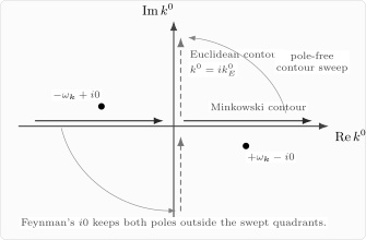
The Feynman prescription places the positive-energy pole below the real axis and the negative-energy pole above it. Wick rotation deforms the loop-energy contour to the imaginary axis without crossing poles.

For external momenta one must also translate invariants carefully. In the common analytic domain,

$$q_E^2=-q_M^2$$

for the corresponding invariant. To approach a physical Feynman amplitude, the continuation is

$$q_E^2\longrightarrow -q_M^2-i0.$$

Thus the parameter denominator becomes $m^2-x(1-x)q_M^2-i0$, which fixes the branch of the logarithm across the two-particle threshold. The rest of this page stays Euclidean unless the contour or continuation is stated explicitly.

Schwinger parameters

The simplest denominator identity is the Laplace transform

$$\boxed{ {1\over A}=\int_0^\infty ds\,e^{-sA}, \qquad \operatorname{Re}A>0. }$$

For the Euclidean propagator, $A=k^2+m^2$ is positive, so this representation is directly convergent:

$${1\over k^2+m^2}=\int_0^\infty ds\,e^{-s(k^2+m^2)}.$$

The parameter $s$ is often called Schwinger proper time. Its dimension is

$$[s]=(\text{mass})^{-2},$$

so small $s$ probes large momenta and large $s$ probes small momenta. This is already a useful diagnostic: ultraviolet divergences appear as singular behavior near $s=0$, while infrared divergences appear as singular behavior near $s=\infty$.

The general identity is

$$\boxed{ {1\over A^n}={1\over \Gamma(n)}\int_0^\infty ds\,s^{n-1}e^{-sA}, \qquad n>0. }$$

For positive real $A$, it follows from the substitution $u=sA$ in the gamma-function integral

$$\Gamma(n)=\int_0^\infty du\,u^{n-1}e^{-u}.$$

Both sides are analytic for $\operatorname{Re}A>0$, so the same identity holds there with $A^{-n}=\exp[-n\operatorname{Log}A]$ on the principal branch. The positive-real substitution alone does not justify changing the contour when $A$ is complex; Exercise 1 supplies the continuation argument.

For the relation between Schwinger and Feynman parameters, see Schwartz 2014, Appendix B.1, pp. 822–823. That source writes the Lorentzian exponential $e^{isA_M}$ with $\operatorname{Im}A_M>0$; setting $A_M=iA$ gives the decaying exponential used here.

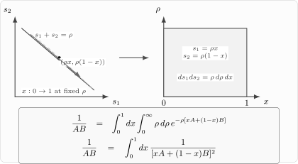
Schwinger parameters exponentiate denominators. For two denominators, the change of variables $(s_1,s_2)=(\rho x,\rho(1-x))$ separates the overall scale $\rho$ from the Feynman parameter $x$; integrating $\rho$ produces the required squared denominator.

The strength of the Schwinger representation is that momentum integrals become Gaussian. For example,

$$\int {d^d k\over(2\pi)^d}\,e^{-s k^2} ={1\over(4\pi s)^{d/2}}.$$

This formula is one of the workhorses of perturbation theory.

Feynman parameters

Schwinger parameters also give the Feynman-parameter formula. Start from

$${1\over AB} = \int_0^\infty ds_1\int_0^\infty ds_2\, e^{-s_1A-s_2B}.$$

Introduce

$$\rho=s_1+s_2, \qquad x={s_1\over s_1+s_2},$$

so that

$$s_1=\rho x, \qquad s_2=\rho(1-x), \qquad 0\le x\le 1, \qquad 0\le \rho<\infty.$$

The Jacobian is

$$ds_1ds_2=\rho\,d\rho\,dx.$$

Therefore

$${1\over AB} = \int_0^1 dx\int_0^\infty \rho\,d\rho\, \exp\{-\rho[xA+(1-x)B]\}.$$

The remaining $\rho$ integral is

$$\int_0^\infty \rho\,d\rho\,e^{-\rho C}={1\over C^2}, \qquad \operatorname{Re}C>0.$$

Thus

$$\boxed{ {1\over AB} =\int_0^1 dx\,{1\over [xA+(1-x)B]^2}. }$$

The square is important. It is the most common place to lose a factor in this calculation.

The general formula is

$$\boxed{ {1\over A_1^{\alpha_1}\cdots A_N^{\alpha_N}} = {\Gamma(\alpha_1+\cdots+\alpha_N)\over \Gamma(\alpha_1)\cdots\Gamma(\alpha_N)} \int_0^1\prod_{i=1}^N dx_i\, {\delta(1-\sum_i x_i)\,x_1^{\alpha_1-1}\cdots x_N^{\alpha_N-1} \over (x_1A_1+\cdots+x_NA_N)^{\alpha_1+\cdots+\alpha_N}}. }$$

For most one-loop two-point and four-point calculations, the two-denominator version is enough.

The scalar bubble

Consider the Euclidean bubble integral

$$I_E(q)=\int {d^d k\over(2\pi)^d}\, {1\over (k^2+m^2)[(q-k)^2+m^2]}.$$

Use the Feynman-parameter formula with

$$A=k^2+m^2, \qquad B=(q-k)^2+m^2.$$

Then

$$I_E(q)=\int_0^1 dx\int {d^d k\over(2\pi)^d} {1\over [x(k^2+m^2)+(1-x)((q-k)^2+m^2)]^2}.$$

The denominator is

$$\begin{aligned} x(k^2+m^2)&+(1-x)((q-k)^2+m^2) \\ &=k^2-2(1-x)q\cdot k+(1-x)q^2+m^2 \\ &=(k-(1-x)q)^2+m^2+x(1-x)q^2. \end{aligned}$$

Define

$$\ell=k-(1-x)q, \qquad \Delta(x,q)=m^2+x(1-x)q^2.$$

If the regulator preserves translation invariance, the shift $k\mapsto\ell$ is harmless, and

$$\boxed{ I_E(q)=\int_0^1 dx\int {d^d\ell\over(2\pi)^d} {1\over [\ell^2+\Delta(x,q)]^2}. }$$

Follow the chosen momentum flow in the upper diagram, then the denominator combination in the panel below. Both internal arrows point from left to right; the downward arrow denotes the algebraic parameterization step.

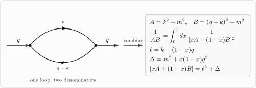
The arrows assign loop momenta, so $q=k+(q-k)$ at both vertices. In the Euclidean domain $m^2>0$ and $0\leq x\leq1$, the parameter shift gives $\Delta=m^2+x(1-x)q^2>0$. Applying this shift inside the integral requires the translation-invariant regulator stated above. The diagram is schematic and not to scale; all parameter identities are derived in the adjacent text.

This is the basic reduction: a two-propagator loop has become a one-parameter family of rotationally invariant Gaussian integrals.

Gaussian momentum integration

The Schwinger representation gives a compact master formula. Initially take $n>0$ real and $\Delta>0$, and start with

$$J_n(\Delta)=\int {d^d\ell\over(2\pi)^d}\,{1\over(\ell^2+\Delta)^n}.$$

At positive integer $d$, this is an ordinary convergent Euclidean integral when $0<d<2n$. Its radial integrand behaves as $r^{d-1}$ at the origin and $r^{d-1-2n}$ at infinity. Continuing the radial expression in $d$ therefore starts in the strip $0<\operatorname{Re}d<2n$; the Gaussian calculation below is justified there before further analytic continuation.

Using

$${1\over(\ell^2+\Delta)^n} ={1\over\Gamma(n)}\int_0^\infty ds\,s^{n-1}e^{-s(\ell^2+\Delta)},$$

we get

$$J_n(\Delta) ={1\over\Gamma(n)}\int_0^\infty ds\,s^{n-1}e^{-s\Delta} \int {d^d\ell\over(2\pi)^d}e^{-s\ell^2}.$$

Since

$$\int {d^d\ell\over(2\pi)^d}e^{-s\ell^2} ={1\over(4\pi s)^{d/2}},$$

we find

$$J_n(\Delta) ={1\over(4\pi)^{d/2}}{1\over\Gamma(n)} \int_0^\infty ds\,s^{n-1-d/2}e^{-s\Delta}.$$

The final integral is another gamma function:

$$\boxed{ \int {d^d\ell\over(2\pi)^d}\,{1\over(\ell^2+\Delta)^n} = {1\over(4\pi)^{d/2}} {\Gamma(n-d/2)\over\Gamma(n)} \Delta^{d/2-n}. }$$

The right-hand side supplies a meromorphic continuation in $d$. Outside the convergence strip it defines the dimensionally regularized expression rather than the value of a convergent unregulated integral. The case $\Delta=0$ requires separate treatment: its radial power $r^{d-1-2n}$ cannot converge at both endpoints for any $d$. The scaleless-integral prescription in dimensional regularization is not an ordinary convergent integral.

The radial Gamma integral and the two common definitions of the dimensional regulator appear in Schwartz 2014, Appendix B.3.2, pp. 826–827.

For the scalar bubble in four dimensions, $n=2$ and $d=4$, so the gamma function contains

$$\Gamma(2-d/2)=\Gamma(0),$$

which is a logarithmic ultraviolet divergence.

In this lesson, put $d=4-\epsilon$ and insert a scale $\mu$ to keep the integral dimensionless. The dimensionally regulated amplitude calculation uses $d=4-2\epsilon$ instead; its $1/\epsilon$ pole is the same pole as the $2/\epsilon$ below after translating the regulator parameter. Expanding the master formula gives

$$\mu^\epsilon\int {d^{4-\epsilon}\ell\over(2\pi)^{4-\epsilon}}\, {1\over(\ell^2+\Delta)^2} ={1\over16\pi^2} \left[ {2\over\epsilon}-\gamma_E+\log4\pi +\log{\mu^2\over\Delta}+O(\epsilon) \right].$$

The pole $2/\epsilon$ is the dimensional-regularization counterpart of the logarithm of a hard cutoff. Defining instead $d=4-2\epsilon$ replaces $2/\epsilon$ by $1/\epsilon$; the two forms encode the same singularity.

Hard cutoff and the coefficient of the logarithm

It is often useful to see the same logarithm with an explicit cutoff. In four Euclidean dimensions,

$$d^4\ell=2\pi^2\ell^3d\ell.$$

If the cutoff is imposed on the shifted momentum $\ell$, then

$$\begin{aligned} J_2^\Lambda(\Delta) &=\int_{|\ell|<\Lambda}{d^4\ell\over(2\pi)^4}\,{1\over(\ell^2+\Delta)^2} \\ &={1\over8\pi^2}\int_0^\Lambda d\ell\,{\ell^3\over(\ell^2+\Delta)^2}. \end{aligned}$$

Set $u=\ell^2$, so $\ell^3d\ell={1\over2}u\,du$. Then

$$J_2^\Lambda(\Delta) ={1\over16\pi^2}\int_0^{\Lambda^2}du\,{u\over(u+\Delta)^2}.$$

Since

$${u\over(u+\Delta)^2}={1\over u+\Delta}-{\Delta\over(u+\Delta)^2},$$

we obtain

$$\boxed{ J_2^\Lambda(\Delta) ={1\over16\pi^2} \left[ \log{\Lambda^2+\Delta\over\Delta} -{\Lambda^2\over\Lambda^2+\Delta} \right]. }$$

For $\Lambda^2\gg\Delta$,

$$J_2^\Lambda(\Delta) ={1\over16\pi^2}\log{\Lambda^2\over\Delta} +\text{nonlogarithmic terms}.$$

The displayed finite terms belong to this particular spherical cutoff in $\ell$. A cutoff imposed before shifting the original loop momentum can change those terms, but not the logarithmic coefficient.

Thus the bubble has leading logarithm

$$\boxed{ I_E(q) ={1\over16\pi^2}\int_0^1 dx\, \log{\Lambda^2\over m^2+x(1-x)q^2} +\text{nonlogarithmic terms}. }$$

For $m^2$ and $q^2$ much smaller than $\Lambda^2$, introduce any fixed reference scale $\mu_{\mathrm{ref}}$. The cutoff dependence takes the form

$$I_E(q)= {1\over16\pi^2}\log{\Lambda^2\over\mu_{\mathrm{ref}}^2} +\text{terms independent of }\Lambda +O(\Lambda^{-2}).$$

Changing $\mu_{\mathrm{ref}}$ only reshuffles the finite term; the coefficient of the cutoff logarithm is universal.

A massless bubble with $q^2>0$ gives

$$I_E(q) ={1\over16\pi^2}\int_0^1 dx\, \log{\Lambda^2\over x(1-x)q^2}+\cdots ={1\over16\pi^2}\left(\log{\Lambda^2\over q^2}+2\right)+\cdots.$$

The constant $2$ is not universal; the coefficient of the logarithm is.

The endpoints $x=0$ and $x=1$ do not introduce an extra divergence in this Euclidean off-shell integral, because

$$\int_0^1 dx\,\log x=-1.$$

They do, however, mark the regions in which one internal line carries nearly all of the external momentum. In on-shell massless Minkowski problems, such endpoint regions often become genuine soft or collinear singularities. For the present off-shell scalar bubble they only contribute a finite constant.

Regulator-independent data

With a hard cutoff, finite constants and power-suppressed terms depend on the shape of the cutoff. The coefficient of

$$\log{\Lambda^2\over \Delta}$$

in a logarithmically divergent local subgraph is the part that survives as universal RG data. This is why the next pages track logarithmic coefficients rather than the full cutoff-dependent integral.

Relation to the φ⁴ vertex

For a Euclidean scalar theory

$$\mathcal L_E={1\over2}(\partial\phi)^2+{1\over2}m^2\phi^2+{\lambda_0\over4!}\phi^4,$$

the one-loop correction to the four-point vertex contains bubble integrals of the type just computed. In one channel, suppressing overall sign conventions from expanding $e^{-S_{\mathrm{int}}}$, the magnitude of the correction is proportional to

$${\lambda_0^2\over2}I_E(q),$$

where the factor $1/2$ is the symmetry factor for the bubble in that channel. The full four-point function has the three channels usually called $s$, $t$, and $u$.

The important point for renormalization is that the logarithmic part is local in the ultraviolet. At large loop momentum,

$${1\over(k^2+m^2)[(q-k)^2+m^2]} \sim {1\over k^4},$$

so the leading UV behavior does not know the external momentum $q$ or the mass $m$. This is why a local counterterm proportional to $\phi^4$ can absorb the divergence.

More explicitly, in the momentum window

$$Q\ll |k|\ll \Lambda,$$

where $Q$ represents any external momentum or mass scale, the integral reduces to

$$\int_Q^\Lambda {d^4k\over(2\pi)^4}{1\over k^4} ={1\over8\pi^2}\log{\Lambda\over Q} ={1\over16\pi^2}\log{\Lambda^2\over Q^2}.$$

That is the leading logarithm in its simplest form.

UV and IR in Schwinger language

The bubble can also be written directly in Schwinger form. Starting from

$$I_E(q)=\int_0^1 dx\int {d^d\ell\over(2\pi)^d}{1\over[\ell^2+\Delta(x,q)]^2},$$

use

$${1\over[\ell^2+\Delta]^2}=\int_0^\infty d\rho\,\rho\,e^{-\rho(\ell^2+\Delta)}.$$

Then

$$I_E(q)=\int_0^1 dx\int_0^\infty d\rho\,\rho\,e^{-\rho\Delta(x,q)} {1\over(4\pi\rho)^{d/2}}.$$

In four dimensions,

$$I_E(q)={1\over(4\pi)^2}\int_0^1 dx\int_0^\infty {d\rho\over\rho}\,e^{-\rho\Delta(x,q)}.$$

With a hard momentum cutoff, the ultraviolet end begins at a lower proper-time limit of order $\rho_{\min}=\Lambda^{-2}$. The logarithmic window is therefore

$$\int_{\Lambda^{-2}}^{Q^{-2}}{d\rho\over\rho} =\log{\Lambda^2\over Q^2},$$

where $Q^2$ stands for the mass or external Euclidean invariant that ends the UV regime. If $\Delta=0$, the large-$\rho$ region is unsuppressed and produces an infrared logarithm as well. The same integral can therefore diagnose both ends of momentum space. This is why Schwinger parameters keep returning in effective actions, heat kernels, background fields, and anomalies.

Summary

The main one-loop technology is now in place.

A Minkowski propagator with Feynman prescription can be Wick-rotated to the Euclidean propagator

$${1\over k^2+m^2}.$$

A denominator can be exponentiated as

$${1\over A}=\int_0^\infty ds\,e^{-sA},$$

and products of denominators can be combined by Feynman parameters, for example

$${1\over AB}=\int_0^1 dx\,{1\over[xA+(1-x)B]^2}.$$

The scalar bubble reduces to

$$I_E(q)=\int_0^1 dx\int {d^d\ell\over(2\pi)^d}{1\over[\ell^2+m^2+x(1-x)q^2]^2}.$$

In four dimensions its leading logarithm is

$$I_E(q)={1\over16\pi^2}\int_0^1 dx\, \log{\Lambda^2\over m^2+x(1-x)q^2}+\cdots.$$

The coefficient of the logarithm is the part that renormalization-group equations will organize and resum.

Common pitfalls

The Feynman-parameter formula for two simple denominators has a squared denominator:

$${1\over AB}=\int_0^1 dx\,{1\over[xA+(1-x)B]^2},$$

not a first power.

A shift of loop momentum is automatic in dimensional regularization and in translation-invariant regulators. With a hard cutoff, shifting the integration variable can change power-divergent pieces. For logarithmic divergences in renormalizable theories, the universal log coefficient is unaffected, but power divergences and finite constants can be regulator-dependent.

Euclidean $q^2$ and Minkowski $q^2$ differ by a sign. A formula derived for positive Euclidean $q^2$ must be continued with $q_E^2\to-q_M^2-i0$ to describe timelike Minkowski scattering. Omitting the boundary prescription loses the threshold branch and imaginary part.

The $i0$ prescription is what permits the Wick rotation. Without it, the location of the poles is ambiguous.

Schwinger parameters make ultraviolet and infrared regions look inverted relative to momentum: small proper time means large momentum, while large proper time means small momentum.

Exercises

Exercise 1: Gamma-function representation

Derive the identity

$${1\over A^n}={1\over\Gamma(n)}\int_0^\infty ds\,s^{n-1}e^{-sA}, \qquad \operatorname{Re}A>0,$$

for arbitrary positive real $n$.

Solution

Start from the definition of the gamma function:

$$\Gamma(n)=\int_0^\infty du\,u^{n-1}e^{-u}.$$

First take $A>0$ real and set

$$u=sA, \qquad u^{n-1}=s^{n-1}A^{n-1}, \qquad du=A\,ds.$$

Then

$$\Gamma(n)=\int_0^\infty ds\,A^n s^{n-1}e^{-sA}.$$

Dividing by $A^n\Gamma(n)$ gives

$${1\over A^n}={1\over\Gamma(n)}\int_0^\infty ds\,s^{n-1}e^{-sA}.$$

For complex $A$ with $\operatorname{Re}A>0$, do not identify the ray $u=sA$ with the positive real axis. Instead, on each compact subset of this half-plane, $s^{n-1}e^{-sA}$ and its $A$ derivatives have an integrable exponential bound. The integral is therefore analytic in $A$, as is $A^{-n}$ with the principal logarithm. They agree for $A>0$, so the identity theorem extends the result throughout the half-plane. The conditions $n>0$ and $\operatorname{Re}A>0$ control the lower and upper endpoints respectively.

Exercise 2: Three Feynman parameters

Use Schwinger parameters to derive

$${1\over ABC} =2\int_0^1 dx\int_0^1 dy\int_0^1 dz\, {\delta(1-x-y-z)\over(xA+yB+zC)^3}.$$

Solution

Write

$${1\over ABC}=\int_0^\infty ds_1ds_2ds_3\, \exp[-s_1A-s_2B-s_3C].$$

Introduce

$$\rho=s_1+s_2+s_3, \qquad x_i={s_i\over\rho}, \qquad x_1+x_2+x_3=1.$$

The measure becomes

$$ds_1ds_2ds_3=\rho^2d\rho\,dx_1dx_2dx_3\,\delta(1-x_1-x_2-x_3).$$

Thus

$${1\over ABC}=\int dx_1dx_2dx_3\,\delta(1-\sum_i x_i) \int_0^\infty d\rho\,\rho^2 \exp[-\rho(x_1A+x_2B+x_3C)].$$

Using

$$\int_0^\infty d\rho\,\rho^2e^{-\rho D}={2\over D^3},$$

we get

$${1\over ABC} =2\int dx_1dx_2dx_3\, {\delta(1-x_1-x_2-x_3)\over(x_1A+x_2B+x_3C)^3}.$$

Renaming $(x_1,x_2,x_3)=(x,y,z)$ gives the stated formula.

Exercise 3: Cutoff bubble integral

Evaluate

$$J_2^\Lambda(\Delta)=\int_{|\ell|<\Lambda}{d^4\ell\over(2\pi)^4}{1\over(\ell^2+\Delta)^2}$$

and extract the leading logarithm for $\Lambda^2\gg\Delta$.

Solution

In four Euclidean dimensions,

$$d^4\ell=2\pi^2\ell^3d\ell.$$

Thus

$$J_2^\Lambda(\Delta)={1\over8\pi^2}\int_0^\Lambda d\ell\,{\ell^3\over(\ell^2+\Delta)^2}.$$

Set $u=\ell^2$, so $\ell^3d\ell={1\over2}u\,du$. Then

$$J_2^\Lambda(\Delta)={1\over16\pi^2}\int_0^{\Lambda^2}du\,{u\over(u+\Delta)^2}.$$

Since

$${u\over(u+\Delta)^2}={1\over u+\Delta}-{\Delta\over(u+\Delta)^2},$$

we find

$$J_2^\Lambda(\Delta) ={1\over16\pi^2}\left[ \log{\Lambda^2+\Delta\over\Delta}-{\Lambda^2\over\Lambda^2+\Delta} \right].$$

For $\Lambda^2\gg\Delta$,

$$J_2^\Lambda(\Delta) ={1\over16\pi^2}\log{\Lambda^2\over\Delta}+\text{nonlogarithmic terms}.$$

Exercise 4: Small-momentum expansion

For $m^2>0$ and small Euclidean momentum $q^2\ll m^2$, show that the finite momentum-dependent part of the bubble satisfies

$$I_E(q)-I_E(0)=-{q^2\over96\pi^2m^2}+O(q^4/m^4).$$

Use the logarithmic expression after the cutoff-dependent constant has been subtracted.

Solution

After subtracting the cutoff-dependent constant, the momentum dependence is

$$I_E(q)-I_E(0) =-{1\over16\pi^2}\int_0^1 dx\, \log\left(1+{x(1-x)q^2\over m^2}\right)+O(\Lambda^{-2}).$$

For $q^2\ll m^2$,

$$\log(1+y)=y+O(y^2),$$

so

$$I_E(q)-I_E(0) =-{1\over16\pi^2}{q^2\over m^2}\int_0^1 dx\,x(1-x)+O(q^4/m^4).$$

But

$$\int_0^1 dx\,x(1-x)={1\over6}.$$

Therefore

$$I_E(q)-I_E(0)=-{q^2\over96\pi^2m^2}+O(q^4/m^4).$$

Exercise 5: Proper-time endpoints

Use Schwinger proper time to identify the UV and IR behavior of

$$K(m)=\int {d^4k\over(2\pi)^4}{1\over(k^2+m^2)^2}.$$

What happens when $m=0$?

Solution

Use

$${1\over(k^2+m^2)^2}=\int_0^\infty ds\,s\,e^{-s(k^2+m^2)}.$$

Then

$$K(m)=\int_0^\infty ds\,s e^{-sm^2}\int {d^4k\over(2\pi)^4}e^{-sk^2}.$$

The Gaussian integral gives

$$\int {d^4k\over(2\pi)^4}e^{-sk^2}={1\over(4\pi s)^2},$$

so

$$K(m)={1\over(4\pi)^2}\int_0^\infty {ds\over s}e^{-sm^2}.$$

The small-$s$ endpoint behaves as $ds/s$, so the integral is logarithmically UV divergent. For $m>0$, the factor $e^{-sm^2}$ suppresses the large-$s$ endpoint, so there is no IR divergence.

If $m=0$, then

$$K(0)={1\over(4\pi)^2}\int_0^\infty {ds\over s},$$

which diverges both at $s=0$ and at $s=\infty$. The same massless integral has both UV and IR logarithmic divergences.

Exercise 6: Finite parameter integral

Show that

$$\int_0^1 dx\,\log[x(1-x)]=-2.$$

Use this to justify the constant term in the massless Euclidean bubble

$$\int_0^1 dx\,\log{\Lambda^2\over x(1-x)q^2} = \log{\Lambda^2\over q^2}+2.$$

Solution

Use

$$\log[x(1-x)]=\log x+\log(1-x).$$

The two integrals are equal by the substitution $u=1-x$:

$$\int_0^1 dx\,\log(1-x)=\int_0^1 du\,\log u.$$

Now

$$\int_0^1 dx\,\log x = [x\log x-x]_0^1=-1,$$

where $x\log x\to0$ as $x\to0^+$. Therefore

$$\int_0^1 dx\,\log[x(1-x)]=-1-1=-2.$$

Thus

$$\int_0^1 dx\,\log{\Lambda^2\over x(1-x)q^2} = \log{\Lambda^2\over q^2}-\int_0^1 dx\,\log[x(1-x)] = \log{\Lambda^2\over q^2}+2.$$

The number $2$ is finite and therefore scheme-dependent in a cutoff calculation; the coefficient of the logarithm is the universal part.

References

• Schwartz, Matthew D. Quantum Field Theory and the Standard Model. Cambridge University Press, 2014. DOI.

Further reading

• Coleman, Sidney. Lectures of Sidney Coleman on Quantum Field Theory. Edited by Bryan Gin-ge Chen, David Derbes, David Griffiths, Brian Hill, Richard Sohn, and Yuan-Sen Ting. World Scientific, 2019. See the lectures on perturbation theory, divergences, and counterterms.
• Srednicki, Mark. Quantum Field Theory. Cambridge University Press, 2007. See Sections 14–20 and 27–29.
• Weinberg, Steven. The Quantum Theory of Fields. Vol. I, Foundations, Cambridge University Press, 1995, Chapters 6 and 12; Vol. II, Modern Applications, Cambridge University Press, 1996, Chapter 18.
• Zinn-Justin, Jean. Quantum Field Theory and Critical Phenomena. 5th ed., Oxford University Press, 2021. See Chapters 1–9.