Sigma-Model Beta Function and Asymptotic Freedom

The nonlinear sigma model is classically simple: a field $\mathbf n(x)$ is constrained to lie on a target sphere, and the action counts how quickly $\mathbf n$ varies in spacetime. Quantum mechanically it is much less innocent. In two dimensions its coupling is classically dimensionless, so the theory sits exactly at the boundary where logarithms can accumulate. The logarithms do accumulate, and their sign is the sign that made the model famous: for $N>2$, the $O(N)$ nonlinear sigma model is asymptotically free.

This page computes the one-loop running in a way that makes the answer geometric. The target-space curvature renormalizes the stiffness of the field. Positive curvature makes the effective stiffness smaller at long distances, so angular fluctuations become stronger in the infrared. Equivalently, the coupling becomes weaker at short distances. The result is

$$\beta(\alpha)=\mu {d\alpha\over d\mu} =-{N-2\over 2\pi}\alpha^2+O(\alpha^3),$$

for the normalization used below. This is the same qualitative mechanism as Yang–Mills asymptotic freedom: a dimensionless coupling is traded for a dynamically generated scale.

Required background. Nonlinear Sigma Models and Constraints supplies the sphere constraint, local coordinates, invariant measure, and slow/fast tangent split used below. Helpful background. Dimensional Transmutation and Mass Gaps explains how an asymptotically free running coupling defines an RG-invariant scale.

Why the coupling is marginal before loops

Normalization and RG variable. We work in two Euclidean dimensions and use

$$S[\mathbf n] ={1\over 2\alpha_0}\int d^2x\,\partial_\mu\mathbf n\cdot\partial_\mu\mathbf n, \qquad \mathbf n^2=1.$$

The coupling $\alpha_0$ is dimensionless in $d=2$. A Wilsonian shell step integrates modes with momenta

$$\Lambda e^{-d\ell}<|k|<\Lambda, \qquad d\ell>0.$$

Thus $d\ell=\log(\Lambda/\mu)$ increases as we move toward the infrared. The beta function in terms of the sliding momentum scale $\mu$ is

$$\beta(\alpha)=\mu {d\alpha\over d\mu}.$$

The action

$$S={1\over2\alpha_0}\int d^dx\,(\partial\mathbf n)^2$$

contains a dimensionless field $\mathbf n$ because of the constraint $\mathbf n^2=1$. Since $[\partial]=1$, the coupling has engineering dimension

$$[\alpha_0]=2-d.$$

Therefore:

• for $d>2$, the sigma-model coupling is irrelevant by power counting;
• for $d<2$, it is relevant;
• for $d=2$, it is classically marginal.

The two-dimensional case is the interesting one. Dimensional analysis does not decide whether the coupling grows or shrinks. One-loop logarithms decide.

A local coordinate expansion already shows why interactions are controlled by $\alpha_0$. Choose a point on the sphere and write the field in terms of $N-1$ local coordinates $\boldsymbol\pi=(\pi^1,\ldots,\pi^{N-1})$:

$$\mathbf n=(\sqrt{1-\boldsymbol\pi^2},\boldsymbol\pi).$$

Then

$$\partial_\mu\mathbf n\cdot\partial_\mu\mathbf n =\partial_\mu\boldsymbol\pi\cdot\partial_\mu\boldsymbol\pi +{(\boldsymbol\pi\cdot\partial_\mu\boldsymbol\pi)^2\over 1-\boldsymbol\pi^2}.$$

So

$$S={1\over2\alpha_0}\int d^2x\, \left[ (\partial\boldsymbol\pi)^2 +(\boldsymbol\pi\cdot\partial_\mu\boldsymbol\pi)^2+ O(\pi^6) \right].$$

If we rescale $\boldsymbol\pi=\sqrt{\alpha_0}\,\boldsymbol\varphi$, the kinetic term for $\boldsymbol\varphi$ is canonical and the first interaction is proportional to $\alpha_0$. Thus weak coupling means a large target sphere in units of the cutoff: nearby fields do not notice the curvature strongly.

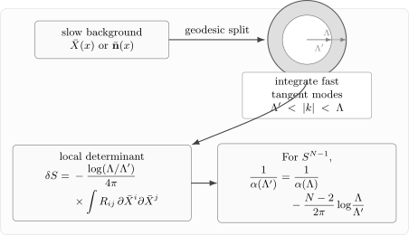
In a Wilsonian step, the slow background field $\bar{\mathbf n}$ is kept fixed while fast tangent fluctuations are integrated over a thin momentum shell. The logarithm comes from the shell integral $\int_{\rm shell} d^2k/k^2$.

Background-field split

The most transparent calculation uses a background-field expansion. It is also the calculation that generalizes from the sphere to any target manifold.

Let the target coordinates be $X^i(x)$ with metric $g_{ij}(X)$. The two-derivative sigma model is

$$S[X]={1\over2\alpha_0}\int d^2x\, g_{ij}(X)\partial_\mu X^i\partial_\mu X^j.$$

We split

$$X(x)=\bar X(x)+\text{fast fluctuation},$$

but the phrase “$+$” is only schematic: on a curved target space, the honest fluctuation is a tangent vector $\xi^i(x)\in T_{\bar X(x)}\mathcal M$. Equivalently, $X(x)$ is reached from $\bar X(x)$ by following the geodesic whose initial tangent is $\xi^i(x)$. These are Riemann normal coordinates around the background.

The covariant derivative acting on the fluctuation is

$$D_\mu\xi^i =\partial_\mu\xi^i+ \Gamma^i{}_{jk}(\bar X)\partial_\mu\bar X^j\xi^k.$$

Use fluctuations of compact support, periodic boundary conditions, or fixed boundary data so that integration by parts has no boundary contribution. The geodesic expansion has a linear term as well as a quadratic term:

$$S[\exp_{\bar X}\xi] =S[\bar X]+S^{(1)}[\xi;\bar X]+S^{(2)}[\xi;\bar X]+O(\xi^3).$$

The first variation is

$$\begin{aligned} S^{(1)} &=-{1\over\alpha_0}\int d^2x\, g_{ij}(\bar X)\xi^i\tau^j(\bar X),\\ \tau^j(\bar X) &=\partial_\mu\partial_\mu\bar X^j +\Gamma^j{}_{kl}(\bar X)\partial_\mu\bar X^k\partial_\mu\bar X^l. \end{aligned}$$

Thus $S^{(1)}$ vanishes on a harmonic background, $\tau^j=0$, but not on an arbitrary slowly varying field. For an off-shell background, the one-loop effective action is defined with the linear source that fixes the mean tangent fluctuation to zero. At the order used here that source cancels $S^{(1)}$; it does not change the quadratic operator. The determinant below is this one-loop contribution, not an assertion that every background solves the classical equation.

The covariant quadratic term is

$$S^{(2)} ={1\over2\alpha_0}\int d^2x\, \left[ g_{ij}(\bar X)D_\mu\xi^iD_\mu\xi^j -R_{ikjl}(\bar X)\partial_\mu\bar X^k\partial_\mu\bar X^l\xi^i\xi^j \right].$$

The first term is the kinetic energy of fast fluctuations. The second term is the tidal effect of target-space curvature. It is the only potential term needed for the one-loop renormalization of the two-derivative action; connection terms in $D_\mu$ complete the same covariant result.

The shell propagator of the fast field, to leading order in the slowly varying background, is

$$\langle \xi^i(k)\xi^j(-k)\rangle_{\rm shell} =\alpha_0\,{g^{ij}(\bar X)\over k^2}.$$

The logarithmic shell integral is

$$\int_{\Lambda e^{-d\ell}<|k|<\Lambda}{d^2k\over(2\pi)^2}{1\over k^2} ={d\ell\over 2\pi}.$$

To first order in the slowly varying background, the Gaussian determinant contributes $\frac12\operatorname{Tr}(K^{-1}V)$. Contracting the two fast fields in the curvature interaction therefore gives

$$\Delta S =-{1\over2}\int d^2x\, R_{kl}(\bar X)\partial_\mu\bar X^k\partial_\mu\bar X^l \int_{\rm shell}{d^2k\over(2\pi)^2}{1\over k^2},$$

where

$$R_{kl}=R^i{}_{kil}$$

is the Ricci tensor of the target space. Hence

$$\boxed{ \Delta S =-{d\ell\over4\pi} \int d^2x\, R_{ij}(\bar X)\partial_\mu\bar X^i\partial_\mu\bar X^j. }$$

This formula is the conceptual heart of the calculation. At one loop, the target metric changes by its Ricci tensor. Positive Ricci curvature decreases the coefficient of the kinetic term as we integrate out shorter distances.

Specializing to the round sphere

For the unit sphere $S^{N-1}$, the Ricci tensor is

$$R_{ij}=(N-2)g_{ij}.$$

Therefore the shell correction is proportional to the original action density:

$$\Delta S =-{N-2\over4\pi}d\ell \int d^2x\,g_{ij}(\bar X) \partial_\mu\bar X^i\partial_\mu\bar X^j.$$

Combining this with

$$S[\bar X]={1\over2\alpha}\int d^2x\, g_{ij}(\bar X)\partial_\mu\bar X^i\partial_\mu\bar X^j,$$

we find the Wilsonian change

$${1\over 2\alpha}\longrightarrow {1\over2\alpha}-{N-2\over4\pi}d\ell.$$

Equivalently,

$$\boxed{ {d\over d\ell}{1\over\alpha}= -{N-2\over2\pi}. }$$

Since $d\ell=-d\log\mu$, this is

$${d\over d\log\mu}{1\over\alpha}= {N-2\over2\pi}.$$

Using

$${d\over d\log\mu}{1\over\alpha} =-{1\over\alpha^2}\mu{d\alpha\over d\mu},$$

we obtain

$$\boxed{ \beta(\alpha)=\mu {d\alpha\over d\mu} =-{N-2\over2\pi}\alpha^2+O(\alpha^3). }$$

For $N>2$, the beta function is negative. The coupling becomes small at high momentum and large at low momentum.

Sign audit

There are two RG “times” in common use. With the momentum scale $\mu$,

$$\beta(\alpha)=\mu{d\alpha\over d\mu}<0$$

means that $\alpha$ decreases toward the ultraviolet. With Wilsonian infrared time $\ell=\log(\Lambda/\mu)$,

$${d\alpha\over d\ell}=+{N-2\over2\pi}\alpha^2+O(\alpha^3),$$

so the same coupling grows as modes are integrated out toward the infrared. These are the same statement written with opposite flow parameters.

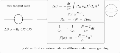
The one-loop correction is geometric: $\Delta S=-(d\ell/4\pi)\int R_{ij}\partial X^i\partial X^j$. For $S^{N-1}$, $R_{ij}=(N-2)g_{ij}$, so positive curvature decreases $1/\alpha$ in the infrared.

Running coupling and generated scale

Let $\alpha_0$ be the coupling defined at the cutoff $\Lambda$. Integrating the one-loop equation gives

$${1\over\alpha(\mu)} ={1\over\alpha_0}-{N-2\over2\pi}\log{\Lambda\over\mu} ={1\over\alpha_0}+{N-2\over2\pi}\log{\mu\over\Lambda}.$$

Thus

$$\boxed{ \alpha(\mu)= {\alpha_0\over 1-{N-2\over2\pi}\alpha_0\log(\Lambda/\mu)} }$$

as long as the denominator remains positive and the coupling is small.

The perturbative coupling becomes order one when

$$1-{N-2\over2\pi}\alpha_0\log{\Lambda\over\mu}\sim 0.$$

This defines the scale

$$\boxed{ M\sim \Lambda\exp\left[-{2\pi\over (N-2)\alpha_0}\right]. }$$

The symbol $M$ should not be interpreted as a perturbative pole. It is the scale where perturbation theory around a fixed direction on the sphere breaks down. Nonperturbatively, the two-dimensional $O(N)$ model with $N>2$ has a mass gap of this order. The coupling $\alpha_0$ has disappeared in favor of the physical scale $M$: this is dimensional transmutation.

The infrared theory therefore does not retain the classical choice of a point on the Mexican-hat minimum. Long-distance angular fluctuations restore $O(N)$, while correlations decay on the scale $M^{-1}$. Symmetry Restoration and Mermin–Wagner Physics gives the finite-volume and infrared arguments; the next page derives the mass scale directly at large $N$.

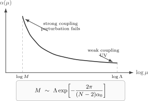
For $N>2$, $\alpha(\mu)$ decreases at short distances and grows toward the infrared. The scale $M\sim\Lambda\exp[-2\pi/((N-2)\alpha_0)]$ marks the end of weak-coupling perturbation theory.

One can package the same result in an RG-invariant form. Define the scale

$$\Lambda_{\sigma}=\mu\exp\left[-{2\pi\over (N-2)\alpha(\mu)}\right]$$

at one loop. Differentiating with respect to $\mu$ and using the beta function gives $d\Lambda_\sigma/d\mu=0$ up to higher-loop corrections. A dimensionless bare coupling has been traded for a physical mass scale.

This is the closest two-dimensional cousin of the QCD story. There is no dimensionful parameter in the classical action, but the quantum theory produces one. The smallness of $M/\Lambda$ at weak bare coupling is nonanalytic in $\alpha_0$; it cannot be seen at any finite order in ordinary perturbation theory.

Field renormalization and the spin structure factor

The constrained vector also requires short-distance renormalization as an operator insertion. Writing $\mathbf n_{\rm bare}=Z_n^{1/2}\mathbf n_{\rm ren}$ does not impose $\mathbf n_{\rm ren}^2=1$: the renormalized insertion and a unit-length target coordinate have different normalization conditions. To obtain a momentum-dependent prediction, we must specify the correlator and its infrared limit as well as its anomalous dimension.

For $N>2$, consider the invariant spin structure factor at nonzero Euclidean momentum,

$$C(p)=\int d^2x\,e^{-ip\cdot x} \langle\mathbf n(x)\cdot\mathbf n(0)\rangle_c, \qquad p=|p_E|>0.$$

The vacuum is at zero temperature and infinite volume, with no symmetry-breaking field. Work in the weak-coupling band $M\ll p\ll\Lambda$. This observable includes all components of $\mathbf n$; the propagator of a transverse chart coordinate alone has a different infrared dependence.

Canceling the infrared regulator

The cancellation can be seen before resumming logarithms. Temporarily add a small source $-h n^1/\alpha_0$, with $h>0$ of mass dimension two, and use $\mathbf n=(\sqrt{1-\boldsymbol\pi^2},\boldsymbol\pi)$. The transverse tree propagator is $\alpha_0/(p^2+h)$. Define

$$\begin{aligned} \Omega(h)&=\int_{|k|<\Lambda}{d^2k\over(2\pi)^2}{1\over k^2+h} ={1\over4\pi}\log\left(1+{\Lambda^2\over h}\right),\\ B(p,h)&=\int{d^2k\over(2\pi)^2} {1\over(k^2+h)((k+p)^2+h)}\\ &={1\over4\pi}\int_0^1{dx\over h+x(1-x)p^2}. \end{aligned}$$

The transverse self-energy contributes $-(N-1)\alpha_0^2\Omega(h)/p^2$ when $p^2\gg h$. The connected longitudinal correlator follows from $n^1=1-\boldsymbol\pi^2/2+\cdots$: its two cross-contractions give $+(N-1)\alpha_0^2 B(p,h)/2$. Consequently, to this order and after discarding terms that vanish with $h/p^2$ and cutoff powers,

$$C(p)={ (N-1)\alpha_0\over p^2} \left[1+\alpha_0\left(-\Omega(h)+{p^2\over2}B(p,h)\right)+\cdots\right].$$

The elementary parameter integral gives

$$B(p,h)={\operatorname{artanh}\!\left(p/\sqrt{p^2+4h}\right) \over\pi p\sqrt{p^2+4h}}.$$

At fixed nonzero $p$, the two infrared logarithms cancel:

$$-\Omega(h)+{p^2\over2}B(p,h) \underset{h\to0}{\longrightarrow} {1\over2\pi}\log{p\over\Lambda}.$$

Thus $p^2C(p)$ starts with $(N-1)\alpha_0[1+\alpha_0\log(p/\Lambda)/(2\pi)+\cdots]$. The transverse term alone retains $\log h$ and does not justify this momentum dependence. The one-loop transverse inverse and RG coefficients used here are given in Zinn-Justin 2021, §§19.11–19.12, pp. 480–481, Eqs. (19.93)–(19.97); the longitudinal contraction and cancellation above supply the invariant observable. Removing $h$ from this invariant perturbative coefficient does not construct a spontaneously ordered massless vacuum.

Running amplitude and anomalous dimension

Use the cutoff RG convention

$$\eta_n(\alpha)=2\gamma_n(\alpha) =-{d\log Z_n\over d\log\Lambda}\bigg|_{\rm ren} ={N-1\over2\pi}\alpha+O(\alpha^2).$$

For the invariant correlator after the infrared limit just described, the connected-function RG equation is

$$\left[\Lambda\partial_\Lambda+\beta(\alpha_0)\partial_{\alpha_0} +\eta_n(\alpha_0)\right]C(p;\alpha_0,\Lambda)=0,$$

up to cutoff-suppressed terms. Before taking that limit there is also a derivative with respect to the source $h$. The source-free equation, dimensional homogeneity and matching at the running momentum give

$$p^2C(p)\simeq A(\alpha(p)) \exp\left[\int_{\alpha_0}^{\alpha(p)} {\eta_n(a)\over\beta(a)}\,da\right], \qquad A(\alpha)=(N-1)\alpha+O(\alpha^2).$$

The matching amplitude runs too. At leading-log order,

$${d\log[p^2C(p)]\over d\log p} ={\beta(\alpha(p))\over\alpha(p)}+\eta_n(\alpha(p)) ={\alpha(p)\over2\pi}.$$

Choose a reference momentum $p_\star$ in the same weak-coupling band and define

$$G_{\rm norm}(p)={C(p)\over p_\star^2C(p_\star)}, \qquad \alpha_\star=\alpha(p_\star).$$

The leading-log prediction is therefore

$$G_{\rm norm}(p)\simeq{1\over p^2} \left({\alpha(p)\over\alpha_\star}\right)^{-1/(N-2)}.$$

Both momenta must remain well above the mass scale and below the cutoff, with weak running couplings. Higher-loop matching, higher-loop running and mass/cutoff power corrections are omitted. A constant normalization of the external field cannot remove the $\alpha(p)$ in the matching amplitude. Nor can this ultraviolet formula be extrapolated into a massless infrared particle pole.

At fixed $g_0=N\alpha_0$ and $N\to\infty$, the exponent tends to zero. The leading saddle has $C(p)=N\alpha_0/(p^2+m^2)$, so the normalized correlator tends to $1/p^2$ when $p,p_\star\gg m$. This agrees with the canonical large-N propagator and Moshe and Zinn-Justin 2003, §3.1, preprint pp. 35–37, Eqs. (3.4)–(3.5) and (3.16), PDF. The source uses a vector of squared length $N$ and coupling $T=g_0$; restoring the unit-vector and canonical-field factors gives the normalization above.

The geometric beta function

For a general target manifold, the same one-loop calculation gives a flow of the target metric. Define the metric that actually multiplies the kinetic term by

$$G_{ij}={g_{ij}\over\alpha}.$$

Then, modulo target-coordinate redefinitions, its Wilsonian flow is

$${dG_{ij}\over d\ell} =-{1\over2\pi}R_{ij}[G] +\text{higher-loop curvature tensors}.$$

This is the seed of the Ricci-flow interpretation of two-dimensional sigma models. It also states the approximation honestly: curvature squared and higher tensor structures enter beyond one loop. If the fixed reference metric is Einstein,

$$R_{ij}=\kappa g_{ij},$$

and only the overall coupling runs at one loop:

$$\beta(\alpha)=-{\kappa\over2\pi}\alpha^2+O(\alpha^3).$$

For the unit sphere $S^{N-1}$,

$$\kappa=N-2.$$

This explains the coefficient in the $O(N)$ beta function without doing a component Feynman-diagram calculation. The coefficient counts curvature, not merely the number of fields. That is why the answer is $N-2$, not $N-1$.

The same formula also explains the special cases:

• $S^1$ is flat, so the perturbative beta function vanishes.
• A positively curved compact target tends to become strongly coupled in the infrared.
• Negative Ricci curvature would reverse the one-loop tendency.

The geometric form is more than pretty language. It is what makes sigma models central in statistical mechanics, string theory, and geometry: the renormalization group acts directly on the target-space metric.

The O(2) exception

For $N=2$, the target space is

$$S^1.$$

We can write

$$n_1=\cos\theta, \qquad n_2=\sin\theta.$$

Then

$$\partial_\mu\mathbf n\cdot\partial_\mu\mathbf n =(\partial_\mu\theta)^2,$$

so the action is exactly Gaussian in the smooth perturbative sector:

$$S={1\over2\alpha}\int d^2x\,(\partial_\mu\theta)^2.$$

The one-loop formula gives zero because $N-2=0$, and in fact the ordinary perturbative beta function vanishes for the free compact boson. “Perturbative” is doing real work here: compactness also permits vortex sectors, which no Taylor expansion around a smooth constant field can produce. Even before vortices are included, the two-dimensional $O(2)$ model has no conventional long-range order. The massless scalar has logarithmic fluctuations:

$$\langle\theta(x)\theta(0)\rangle =-{\alpha\over2\pi}\log{|x|\over a}+\text{constant},$$

where $a$ is a short-distance cutoff. Therefore the order-parameter correlator behaves as

$$\langle e^{i\theta(x)}e^{-i\theta(0)}\rangle =\exp\left[-{1\over2}\langle(\theta(x)-\theta(0))^2\rangle\right] \propto |x|^{-\alpha/(2\pi)}.$$

It decays as a power, not to a nonzero constant. Continuous symmetry is not spontaneously broken in the usual long-range sense. Nonperturbative vortices add another layer and lead to the Berezinskii–Kosterlitz–Thouless phenomenon, but the perturbative message is already visible: flat target space removes the $N-2$ beta function, while infrared fluctuations still destroy a fixed classical direction.

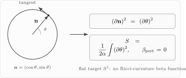
For $O(2)$, $\mathbf n=(\cos\theta,\sin\theta)$ and the perturbative action is a compact free boson. The Ricci curvature of $S^1$ vanishes, so the $N-2$ beta-function coefficient is zero.

A direct component check

It is useful to see where the logarithm lives in ordinary coordinates. Expanding

$$\mathbf n=(\sqrt{1-\boldsymbol\pi^2},\boldsymbol\pi)$$

gives the quartic derivative interaction

$$S_{\rm int} ={1\over2\alpha_0}\int d^2x\, (\boldsymbol\pi\cdot\partial_\mu\boldsymbol\pi)^2+\cdots.$$

After the rescaling $\boldsymbol\pi=\sqrt{\alpha_0}\boldsymbol\varphi$, this becomes

$$S_{\rm int} ={\alpha_0\over2}\int d^2x\, (\boldsymbol\varphi\cdot\partial_\mu\boldsymbol\varphi)^2+ \cdots.$$

A one-loop correction to the two-derivative term comes from contracting two fast $\boldsymbol\varphi$ fields in the shell. The contraction produces

$$\int_{\rm shell}{d^2k\over(2\pi)^2}{1\over k^2} ={d\ell\over2\pi},$$

and the remaining slow fields reconstruct $(\partial\mathbf n)^2$. A component calculation must also include the fact that the local-coordinate field is not itself the globally constrained vector and that the measure/field renormalization contributes. After these pieces are combined, the coefficient is $N-2$.

This separates two coefficients that are easy to conflate. The shortening of the slow vector found on the previous page is

$${1\over2}\langle\boldsymbol\xi^2\rangle_{\rm shell} ={N-1\over4\pi}\alpha\,d\ell,$$

and it controls the one-loop anomalous dimension of the $\mathbf n$ insertion. The change of the two-derivative coupling instead includes the curvature and measure contributions and is proportional to $N-2$. Thus $N-1$ in field renormalization and $N-2$ in the beta function are compatible, not competing answers.

This is a good place to be suspicious of quick diagrammatic arguments. A naive count of transverse fields gives $N-1$, but the correct beta function is governed by the Ricci tensor of $S^{N-1}$, hence $N-2$. The background-field method keeps this covariance manifest and prevents the wrong count from becoming a wrong answer.

Summary

The two-dimensional $O(N)$ nonlinear sigma model is classically scale invariant because its coupling is dimensionless. Quantum fluctuations break this classical scale invariance. In the normalization

$$S={1\over2\alpha}\int d^2x\,(\partial\mathbf n)^2, \qquad \mathbf n^2=1,$$

the one-loop beta function is

$$\beta(\alpha)=-{N-2\over2\pi}\alpha^2+O(\alpha^3).$$

For $N>2$, this is asymptotic freedom: the coupling becomes weak at short distances and strong at long distances. The running coupling is

$$\alpha(\mu)= {\alpha_0\over 1-{N-2\over2\pi}\alpha_0\log(\Lambda/\mu)},$$

and the scale where perturbation theory fails is

$$M\sim\Lambda\exp\left[-{2\pi\over(N-2)\alpha_0}\right].$$

The one-loop correction is geometrically

$$\Delta S=-{d\ell\over4\pi}\int R_{ij}\partial X^i\partial X^j.$$

Thus the beta function is controlled by target-space Ricci curvature. For the sphere, $R_{ij}=(N-2)g_{ij}$. For $S^1$, the curvature vanishes and the perturbative beta function is zero.

Common pitfalls

Confusing the sign of the beta function. With $\beta(\alpha)=\mu d\alpha/d\mu$, asymptotic freedom means $\beta(\alpha)<0$ at small positive $\alpha$. The same statement in Wilsonian infrared time $\ell=\log(\Lambda/\mu)$ is $d\alpha/d\ell>0$.

Counting transverse fields instead of curvature. There are $N-1$ local coordinates on $S^{N-1}$, but the one-loop beta-function coefficient is $N-2$. The former coefficient appears in the field anomalous dimension; the latter is the Ricci curvature of the target sphere.

Taking the perturbative pole literally. The scale $M$ is not a physical Landau pole. It marks the failure of weak-coupling perturbation theory and the onset of nonperturbative mass-gap physics.

Using an anomalous dimension without a matching amplitude. The invariant spin structure factor includes transverse and longitudinal contributions. Its leading-log momentum dependence contains both operator renormalization and the running tree amplitude; a transverse chart propagator with a fixed infrared source cannot be substituted for it.

Treating $O(2)$ as an ordered phase because the beta function vanishes. The perturbative beta function vanishes for the compact free boson, but two-dimensional infrared fluctuations still remove ordinary long-range order. Vortices are nonperturbative and must be treated separately.

Exercises

Exercise 1: deriving the running coupling

Starting from

$$\beta(\alpha)=-b\alpha^2, \qquad b={N-2\over2\pi},$$

solve for $\alpha(\mu)$ in terms of $\alpha_0=\alpha(\Lambda)$. Find the scale $M$ at which the one-loop coupling becomes singular.

Solution

The RG equation is

$$\mu{d\alpha\over d\mu}=-b\alpha^2.$$

Equivalently,

$${d\alpha\over d\log\mu}=-b\alpha^2.$$

Separate variables:

$${d\alpha\over\alpha^2}=-b\,d\log\mu.$$

Integrating from $\Lambda$ to $\mu$ gives

$$-{1\over\alpha(\mu)}+{1\over\alpha_0} =-b\log{\mu\over\Lambda}.$$

Hence

$${1\over\alpha(\mu)} ={1\over\alpha_0}+b\log{\mu\over\Lambda} ={1\over\alpha_0}-b\log{\Lambda\over\mu}.$$

Therefore

$$\alpha(\mu)= {\alpha_0\over 1-b\alpha_0\log(\Lambda/\mu)}.$$

The denominator vanishes at

$$1-b\alpha_0\log{\Lambda\over M}=0,$$

so

$$M=\Lambda\exp\left[-{1\over b\alpha_0}\right] =\Lambda\exp\left[-{2\pi\over(N-2)\alpha_0}\right].$$

Exercise 2: shell integral in two dimensions

Show that

$$\int_{\Lambda e^{-d\ell}<|k|<\Lambda}{d^2k\over(2\pi)^2}{1\over k^2} ={d\ell\over2\pi}+O(d\ell^2).$$

Solution

Use polar coordinates in momentum space:

$$d^2k=k\,dk\,d\varphi.$$

Then

$$\int_{\Lambda e^{-d\ell}}^\Lambda {k\,dk\over(2\pi)^2}{1\over k^2} \int_0^{2\pi}d\varphi ={1\over2\pi} \int_{\Lambda e^{-d\ell}}^\Lambda {dk\over k}.$$

The remaining integral is

$$\log\Lambda-\log(\Lambda e^{-d\ell})=d\ell.$$

Thus

$$\int_{\rm shell}{d^2k\over(2\pi)^2}{1\over k^2} ={d\ell\over2\pi}.$$

Exercise 3: the O(2) model as a free compact boson

Let

$$\mathbf n=(\cos\theta,\sin\theta).$$

Show that

$$(\partial_\mu\mathbf n)^2=(\partial_\mu\theta)^2.$$

Then use the free-boson propagator to show that

$$\langle e^{i\theta(x)}e^{-i\theta(0)}\rangle \propto |x|^{-\alpha/(2\pi)}.$$

Solution

Differentiate $\mathbf n$:

$$\partial_\mu\mathbf n =(-\sin\theta\,\partial_\mu\theta,\cos\theta\,\partial_\mu\theta).$$

Therefore

$$(\partial_\mu\mathbf n)^2 =\sin^2\theta\,(\partial_\mu\theta)^2 +\cos^2\theta\,(\partial_\mu\theta)^2 =(\partial_\mu\theta)^2.$$

The action is

$$S={1\over2\alpha}\int d^2x\,(\partial\theta)^2.$$

The Green function satisfies

$$-{1\over\alpha}\partial^2 G(x)=\delta^{(2)}(x),$$

so at large separation

$$G(x)=\langle\theta(x)\theta(0)\rangle =-{\alpha\over2\pi}\log{|x|\over a}+\text{constant}.$$

For a Gaussian field,

$$\langle e^{i\theta(x)}e^{-i\theta(0)}\rangle =\exp\left[-{1\over2}\langle(\theta(x)-\theta(0))^2\rangle\right].$$

Using

$$\langle(\theta(x)-\theta(0))^2\rangle ={\alpha\over\pi}\log{|x|\over a}+\text{constant},$$

we get

$$\langle e^{i\theta(x)}e^{-i\theta(0)}\rangle \propto |x|^{-\alpha/(2\pi)}.$$

Exercise 4: Ricci curvature and the coefficient N minus two

The unit sphere $S^m$ has Ricci tensor

$$R_{ij}=(m-1)g_{ij}.$$

Use the geometric one-loop correction

$$\Delta S=-{d\ell\over4\pi}\int R_{ij}\partial X^i\partial X^j$$

for the $O(N)$ model. Derive the one-loop beta function.

Solution

For the $O(N)$ model the target is $S^{N-1}$, so

$$m=N-1.$$

The Ricci tensor is therefore

$$R_{ij}=(m-1)g_{ij}=(N-2)g_{ij}.$$

The one-loop correction is

$$\Delta S=-{N-2\over4\pi}d\ell \int d^2x\,g_{ij}\partial_\mu X^i\partial_\mu X^j.$$

The original action is

$$S={1\over2\alpha}\int d^2x\,g_{ij}\partial_\mu X^i\partial_\mu X^j.$$

Thus

$${1\over2\alpha}\to {1\over2\alpha}-{N-2\over4\pi}d\ell,$$

or

$${d\over d\ell}{1\over\alpha}=-{N-2\over2\pi}.$$

Since $d\ell=-d\log\mu$,

$${d\over d\log\mu}{1\over\alpha}={N-2\over2\pi}.$$

Using

$${d\over d\log\mu}{1\over\alpha}=-{1\over\alpha^2}\beta(\alpha),$$

we obtain

$$\beta(\alpha)=-{N-2\over2\pi}\alpha^2.$$

Exercise 5: matching the invariant spin correlator

Let

$$F(p)={p^2C(p)\over p_\star^2C(p_\star)}, \qquad F(p_\star)=1,$$

where $C$ is the invariant structure factor defined above. Its leading-log matching amplitude is $A(\alpha)=(N-1)\alpha$, and its RG transport factor is $\exp[\int\eta_n/\beta\,d\alpha]$, with

$$\eta_n(\alpha)={N-1\over2\pi}\alpha, \qquad \beta(\alpha)=-{N-2\over2\pi}\alpha^2.$$

Derive $G_{\rm norm}(p)=F(p)/p^2$ and check its large-$N$ limit at fixed $g_0=N\alpha_0$. Why is $d\log F/d\log p=-\eta_n$ not the RG equation for this observable?

Solution

The amplitude ratio contributes one power of the running coupling. Including operator transport gives

$$F(p)={\alpha(p)\over\alpha_\star} \exp\left[\int_{\alpha_\star}^{\alpha(p)} {\eta_n(\alpha)\over\beta(\alpha)}\,d\alpha\right].$$

Since $\eta_n/\beta=-(N-1)/[(N-2)\alpha]$,

$$\log F(p)=\left(1-{N-1\over N-2}\right) \log{\alpha(p)\over\alpha_\star} =-{1\over N-2}\log{\alpha(p)\over\alpha_\star}.$$

Therefore

$$G_{\rm norm}(p) ={1\over p^2} \left({\alpha(p)\over\alpha_\star}\right)^{-1/(N-2)}.$$

Equivalently,

$${d\log F\over d\log p}={\beta(\alpha)\over\alpha}+\eta_n(\alpha) ={\alpha\over2\pi}.$$

The proposed $-\eta_n$ equation both omits the running amplitude and reverses the connected-function transport sign. At fixed $g_0$ and fixed weak-coupling momentum ratios, $\alpha(p)/\alpha_\star$ has a finite large-$N$ limit, while the exponent $-1/(N-2)$ vanishes. Thus $G_{\rm norm}\to1/p^2$ in the ultraviolet, consistent with the massive large-$N$ saddle up to mass-suppressed corrections. The transverse tree factor alone does not establish this invariant result; the infrared cancellation requires the longitudinal contraction as well.

References

• E. Brézin and J. Zinn-Justin, “Renormalization of the Nonlinear Sigma Model in $2+\epsilon$ Dimensions—Application to the Heisenberg Ferromagnets,” Physical Review Letters 36 (1976) 691–694, doi:10.1103/PhysRevLett.36.691.
• D. Friedan, “Nonlinear Models in $2+\epsilon$ Dimensions,” Physical Review Letters 45 (1980) 1057–1060, doi:10.1103/PhysRevLett.45.1057.
• M. Moshe and J. Zinn-Justin, “Quantum Field Theory in the Large N Limit: A Review,” Physics Reports 385 (2003), 69–228, doi:10.1016/S0370-1573(03)00263-1, Open PDF, arXiv v1.
• A. M. Polyakov, “Interaction of Goldstone Particles in Two Dimensions. Applications to Ferromagnets and Massive Yang–Mills Fields,” Physics Letters B 59 (1975) 79–81, doi:10.1016/0370-2693(75)90161-6.
• J. Zinn-Justin, Quantum Field Theory and Critical Phenomena, 5th ed. (Oxford University Press, 2021), doi:10.1093/oso/9780198834625.001.0001.

Further reading

• A. M. Polyakov, Gauge Fields and Strings, Contemporary Concepts in Physics, Vol. 3, Harwood Academic Publishers, Chur, 1987.
• S. Weinberg, The Quantum Theory of Fields, Volume II: Modern Applications, Cambridge University Press, Cambridge, 1996.
• A. Zee, Quantum Field Theory in a Nutshell, 2nd ed., Princeton University Press, Princeton, 2010.