Propagation of Singularities for Hyperbolic Fields

For a scalar operator of real principal type, a singularity that is already present cannot disappear at one isolated point of a source-free characteristic ray, nor can a new one appear there. If $Pu=f$, the part of $\operatorname{WF}(u)$ outside $\operatorname{WF}(f)$ is transported by the Hamilton flow of the principal symbol. For Klein–Gordon fields, the resulting phase-space curves project to null geodesics.

That statement is local and deliberately narrow. It stops at a source wavefront, requires a replacement theorem at a boundary or radial set, and does not determine amplitudes, decay, geodesic completeness, or the existence or positivity of a quantum state. This page states the theorem precisely, explains its positive-commutator mechanism, works through a retarded point source, and shows why a caustic breaks a coordinate amplitude without ending the wavefront.

Throughout this page, source-free means microlocally source-free: the characteristic segment is disjoint from $\operatorname{WF}(f)$. The function or distribution $f$ may be nonzero there, provided it is smooth in the covector directions under discussion.

Required background. Microlocal calculus for quantum fields supplies wavefront sets and elliptic regularity; Green-hyperbolic operators and causal propagators supplies the globally defined retarded and advanced operators used in the application.

Helpful background. Wavefront-set products, pullbacks, and pushforwards supplies the primed-kernel convention and kernel-composition rule; domains, signatures, supports, and regularity fixes the distributional domain; propagation of the Hadamard property gives the complete physical deployment.

The chapter overview supplies three complementary guides: the dependency map places this theorem between wavefront calculus and microlocal spectrum conditions, the hypothesis–conclusion table separates local regularity from global state claims, and the failure map records what breaks when a hypothesis is removed.

For a direct route, begin with the Hamilton geometry, then read the propagation theorem and the Klein–Gordon specialization. The point-source calculation is the main QFT application, while the caustic test and scope qualifications prevent the most common overclaims.

Characteristic covectors and Hamilton flow

Let $X$ be a smooth manifold and let

$$P\in\Psi^r_{\mathrm{cl}}(X)$$

be a properly supported scalar classical pseudodifferential operator. Its principal symbol $p(x,k)$ is homogeneous of degree $r$ in the nonzero cotangent variable $k$. The zero section must be removed before discussing characteristic directions:

$$\operatorname{Char}(P) = \left\{ (x,k)\in T^*X\setminus 0:p(x,k)=0 \right\}.$$

The operator is of real principal type here when $p$ is real and

$$\mathrm dp\neq0 \quad\text{on}\quad \operatorname{Char}(P).$$

The qualification $k\neq0$ matters. For the quadratic Klein–Gordon symbol, both $p$ and $\mathrm dp$ vanish at the zero covector, but that covector is never part of a wavefront set.

In canonical coordinates $(x^a,k_a)$, the Hamilton vector field is

$$H_p = \frac{\partial p}{\partial k_a} \frac{\partial}{\partial x^a} - \frac{\partial p}{\partial x^a} \frac{\partial}{\partial k_a}.$$

A bicharacteristic is an integral curve $\gamma(s)=(x(s),k(s))$ of $H_p$ in $T^*X\setminus0$. Since

$$\frac{\mathrm d}{\mathrm ds}p(\gamma(s)) =H_pp =\{p,p\} =0,$$

a bicharacteristic that starts in $\operatorname{Char}(P)$ remains there. The parametrization is less important than the orbit. If $q=ap$ on the conic region of interest, where $a$ is smooth, real, nonvanishing, and homogeneous of degree zero, then $q$ is another real principal symbol of order $r$ and

$$H_{ap}=aH_p+pH_a,$$

so $H_{ap}=aH_p$ on $p=0$: the same characteristic curves are merely reparametrized, with orientation reversed if $a<0$.

The real-principal-type propagation theorem

Three microlocal statements play different roles. Pseudolocality says

$$\operatorname{WF}(Pu) \subset \operatorname{WF}(u).$$

Elliptic regularity supplies the reverse inclusion away from the characteristic set,

$$\operatorname{WF}(u) \subset \operatorname{WF}(Pu) \cup \operatorname{Char}(P).$$

Propagation then determines what happens along the remaining characteristic directions.

Propagation of singularities

Let $P$ have the real-principal-type hypotheses above, let $u\in\mathcal D'(X)$, and write $Pu=f$. Then

$$\operatorname{WF}(u) \setminus \operatorname{WF}(f) \subset \operatorname{Char}(P),$$

and this relative wavefront set is invariant under $H_p$. Equivalently, if a connected bicharacteristic segment satisfies

$$\gamma(I) \subset \operatorname{Char}(P) \setminus \operatorname{WF}(f),$$

then exactly one of the following holds:

$$\gamma(I)\subset\operatorname{WF}(u), \qquad\text{or}\qquad \gamma(I)\cap\operatorname{WF}(u)=\varnothing.$$

This is Duistermaat and Hörmander 1972, § 6.1, Theorem 6.1.1, printed p. 196 (PDF). The phrase “maximally extended” always means maximally extended inside the stated source-free conic region. It does not assert that the projected geodesic is complete. An endpoint of that source-free segment may meet $\operatorname{WF}(f)$, leave the coordinate or microlocal region, reach a physical boundary or radial set, or become inextendible with the spacetime itself.

There is also a Sobolev-strength refinement. A distribution $v$ is microlocally $H^s$ at $(x,k)$ when some properly supported order-zero pseudodifferential operator $A$, elliptic at $(x,k)$, makes $Av$ locally $H^s$; the Sobolev wavefront set $\operatorname{WF}^s(v)$ records where this fails. For an operator $P$ of order $r$,

$$\operatorname{WF}^s(u) \setminus \operatorname{WF}^{s-r+1}(Pu)$$

is a union of bicharacteristics in $\operatorname{Char}(P)\setminus\operatorname{WF}^{s-r+1}(Pu)$. Equivalently, if $Pu$ is microlocally $H^{s-r+1}$ along a characteristic segment and $u$ is microlocally $H^s$ at one point, then $H^s$ regularity propagates throughout that segment. The source hypothesis is one derivative better than the natural mapping $P:H^s\to H^{s-r}$. Applying the result at every Sobolev order recovers the ordinary $C^\infty$ wavefront theorem; neither statement says that a singularity keeps one fixed amplitude or distributional order.

Why the theorem works

The proof turns Hamilton geometry into an energy estimate.

1. Choose pseudodifferential cutoffs that localize to a short tube around the bicharacteristic and order them in the direction of $H_p$.
2. Commute $P$ with a self-adjoint microlocalizer. The principal symbol of the commutator contains the derivative of the cutoff along the flow, $H_p a$.
3. Arrange the sign of that derivative so the commutator controls the desired Sobolev norm at the next point of the tube, with errors supported where regularity is already known or where the source is controlled.
4. Iterate the estimate along overlapping tubes. Repeating it for all Sobolev orders gives the $C^\infty$ wavefront statement.

This explains both the power and the limit of the result. The principal symbol fixes the route; lower-order terms enter amplitudes and, at radial sets discussed below, subprincipal data enter regularity thresholds. A commutator estimate propagates from one known microlocally regular point in a chosen Hamilton direction; applying it to the reversed direction gives the two-sided, all-or-none conclusion on the bicharacteristic segment.

Why Klein–Gordon bicharacteristics are null geodesics

Let $(M,g)$ have the site-wide signature $(+---)$ and consider

$$P=\Box_g+m^2+\xi R.$$

With the site’s Fourier convention $\partial_a\mapsto-ik_a$, the raw order-two differential symbol differs by an overall sign from $g^{ab}k_ak_b$. By the rescaling observation above, it is convenient to use the Hamiltonian representative

$$h(x,k)=\frac12g^{ab}(x)k_ak_b.$$

Its characteristic set is the nonzero null cone. Hamilton’s equations are

$$\dot x^a =g^{ab}k_b =k^{\sharp a}, \qquad \dot k_a =- \frac12 \partial_a g^{bc} k_bk_c.$$

These equations are equivalent to

$$\nabla_{\dot x}\dot x=0, \qquad \nabla_{\dot x}k=0.$$

Because $h=0$ is preserved, $g(\dot x,\dot x)=0$. The projection $x(s)$ is therefore an affinely parametrized null geodesic and $k$ is parallel transported along it. A bicharacteristic is the lifted phase-space curve $(x(s),k(s))$; the null geodesic is only its base-space projection.

The terms $m^2$ and $\xi R$ have order zero. They can change transport amplitudes, smooth tails, and the global Green operator, but not the local characteristic cone. This resolves a common apparent paradox: the momentum-space propagator has its finite-scale pole on the timelike mass shell, whereas the position-space wavefront set is a different, conic object that probes ultraviolet directions. At large covector scale the massive shell approaches the null cone selected by the homogeneous principal symbol.

A 1+1-dimensional null-front check

In $1+1$ Minkowski spacetime,

$$u(t,x)=\delta(t-x)$$

satisfies $(\partial_t^2-\partial_x^2)u=0$. Its wavefront set is

$$\operatorname{WF}(u) = \left\{ (t,x;\lambda,-\lambda): t=x,\ \lambda\neq0 \right\}.$$

For $h=(k_t^2-k_x^2)/2$, Hamilton’s equations give

$$\dot t=k_t, \qquad \dot x=-k_x, \qquad \dot k=0.$$

Starting from $k=\lambda(1,-1)$ therefore moves tangent to $t-x=0$ and keeps the covector fixed. Both signs of $\lambda$ occur. The field equation transports either orientation; it does not choose a positive-frequency half-cone.

A retarded point source

Global hyperbolicity enters now, not in the local theorem. For a formally self-adjoint normally hyperbolic $P$, the Green operators on smooth compact sources extend to compactly supported distributions $F\in\mathcal E'(M)$ by duality:

$$\left\langle G_{\mathrm{ret}}F,\phi \right\rangle = \left\langle F,G_{\mathrm{adv}}\phi \right\rangle, \qquad \phi\in C_c^\infty(M).$$

For a non-self-adjoint operator, the advanced operator of the formal adjoint appears on the right. This definition is what licenses the notation $G_{\mathrm{ret}}\delta_y$; it is not a naive product of two arbitrary distributions.

For the massless wave operator in $3+1$ Minkowski spacetime, a point source at the origin gives, away from the vertex $r=0$,

$$G_{\mathrm{ret}}\delta_0(t,\mathbf x) = \frac{\delta(t-r)}{4\pi r}, \qquad r=\lvert\mathbf x\rvert, \qquad t>0.$$

The future light cone is the hypersurface $F=t-r=0$. Its nonzero conormals are

$$\lambda\,\mathrm dF = \lambda \left( \mathrm dt- \widehat{\mathbf x}\mathbin{\cdot}\mathrm d\mathbf x \right), \qquad \lambda\neq0.$$

They are characteristic because

$$g^{-1}(\mathrm dF,\mathrm dF) =1-\lvert\widehat{\mathbf x}\rvert^2 =0.$$

Raising the covector gives a tangent proportional to $\partial_t+\widehat{\mathbf x}\cdot\nabla$, so Hamilton flow follows the outgoing null generator. Retarded support chooses the future light cone in base space, but the conormal parameter still has both signs $\lambda>0$ and $\lambda<0$. Retarded is not a synonym for positive frequency.

The point source has

$$\operatorname{WF}(\delta_0) = \left\{ (0,\eta):\eta\neq0 \right\}.$$

At that source covector the propagation theorem makes no comparison across the vertex. Away from it, the singular directions are forced to follow the future-supported null flow. Locally in a convex normal neighborhood, a massive or curved-spacetime Green function may also have a smooth tail in the open timelike interior away from the direct null front. Globally, lensing or conjugate points can send additional null wavefront branches to points in that interior. By contrast, if $f\in C_c^\infty(M)$, then $G_{\mathrm{ret}}f$ is smooth. Compact support alone does not launch a wavefront—nonsmooth source covectors do.

The point-source calculation is one slice of a two-point Green-kernel relation. The next section makes that relation precise.

Green kernels and distinguished parametrices

Let $K\in\mathcal D'(M\times M)$ be a kernel and use the primed convention

$$\operatorname{WF}'(K) = \left\{ (x,k;y,\ell): (x,k;y,-\ell)\in\operatorname{WF}(K) \right\}.$$

Write

$$\Delta^* = \left\{ (x,k;x,k):k\neq0 \right\}$$

for the nonzero diagonal relation. Put $\mathcal N=\operatorname{Char}(P)$. Write $(x,k)\sim(y,\ell)$ only when $(x,k),(y,\ell)\in\mathcal N$ lie on the same $H_p$ orbit. For a normally hyperbolic scalar operator, this means that $k$ and $\ell$ are nonzero null cotangents, their metric duals are tangent to the connecting null geodesic, and they are related by parallel transport. Define

$$\begin{aligned} \mathcal C_{\mathrm{ret}} &= \left\{ (x,k;y,\ell): (x,k)\sim(y,\ell),\ x\in J^+(y) \right\},\\ \mathcal C_{\mathrm{adv}} &= \left\{ (x,k;y,\ell): (x,k)\sim(y,\ell),\ x\in J^-(y) \right\},\\ \mathcal C &= \mathcal C_{\mathrm{ret}} \cup \mathcal C_{\mathrm{adv}}. \end{aligned}$$

For a normally hyperbolic operator on a boundaryless globally hyperbolic spacetime, the exact kernel relations are

$$\begin{aligned} \operatorname{WF}'(G_{\mathrm{ret}}) &=\Delta^*\cup\mathcal C_{\mathrm{ret}},\\ \operatorname{WF}'(G_{\mathrm{adv}}) &=\Delta^*\cup\mathcal C_{\mathrm{adv}},\\ \operatorname{WF}'(E) &=\mathcal C, \qquad E=G_{\mathrm{ret}}-G_{\mathrm{adv}}. \end{aligned}$$

The last equality means that the noncharacteristic diagonal inverse singularities cancel; the null diagonal directions remain as part of $\mathcal C$. A current vector-bundle refinement, including the transported fibre polarization, is given in Fewster 2026, equations (1.4)–(1.7), pp. 1–2, and Theorem 1.1, pp. 3–4 (preprint PDF).

A parametrix is an inverse modulo a smoothing operator. Microlocally in an elliptic region, any two parametrices differ by a smoothing operator. The diagonal singularity is imposed by inversion; away from the diagonal, propagation permits characteristic flow-outs. Four standard distinguished choices organize those flow-outs:

• The exact $G_{\mathrm{ret}}$ and $G_{\mathrm{adv}}$ have future and past support in base space. The corresponding distinguished retarded and advanced parametrix classes are characterized modulo smooth kernels by $\operatorname{WF}'\subset\Delta^*\cup\mathcal C_{\mathrm{ret}}$ or $\operatorname{WF}'\subset\Delta^*\cup\mathcal C_{\mathrm{adv}}$ and contain both covector time orientations. Adding a smooth kernel can destroy causal support without changing the microlocal class.
• The Feynman choice propagates the future-directed covector component forward and the past-directed component backward; the anti-Feynman choice reverses that pairing.

These are microlocal inverse conditions, not state constructions. A Feynman parametrix does not by itself supply positivity or a preferred state, and retarded support does not impose a frequency sign. Duistermaat and Hörmander construct and distinguish these parametrices in Duistermaat and Hörmander 1972, §§ 6.5–6.6 (PDF).

For a bisolution, applying propagation in the two variables transports components whose two slot covectors are both nonzero. It does not by itself exclude partial-zero elements

$$(x,k;y,0), \qquad (x,0;y,\ell).$$

The complete Hadamard argument combines the local cone, both field equations, and a support-moving time-slice reconstruction with kernel composition. The complete Cauchy-band deployment works through that missing step. The local Hadamard condition selects the allowed frequency orientation; the commutator fixes the antisymmetric part; positivity remains separate state data. See Radzikowski 1996, Theorem 5.1 and the propagation argument on printed pp. 546–552.

A caustic is a projection failure, not a wavefront endpoint

A Lagrangian distribution is locally an oscillatory integral whose phase parametrizes a conic Lagrangian submanifold of the nonzero cotangent bundle. A geometric-optics chart tries to express that submanifold with an eikonal phase and branchwise transport amplitudes. The chart can fail even while the lifted phase-space geometry remains smooth.

Here is an exact null example that keeps the zero section out of the calculation. The symbols $(t,x,z)$ are base coordinates; $(\mu,\lambda)$ are homogeneous phase variables; $\lambda>0$ selects one conic sheet and sets the covector scale. The ratio $s=\mu/\lambda$ labels neighboring rays, while varying $t$ at fixed $s$ follows one ray. In $1+2$ Minkowski spacetime with metric $\mathrm dt^2-\mathrm dx^2-\mathrm dz^2$, use the degree-one homogeneous phase

$$\Phi(t,x,z;\mu,\lambda) :=x\mu+z\lambda -t\sqrt{\mu^2+\lambda^2} -\frac{\mu^3}{3\lambda^2}.$$

With $s=\mu/\lambda$, the two fiber-critical equations give

$$\begin{aligned} x&=\frac{ts}{\sqrt{1+s^2}}+s^2,\\ z&=\frac{t}{\sqrt{1+s^2}}-\frac{2s^3}{3}. \end{aligned}$$

Thus the base point and its covector are

$$\begin{aligned} q(t,s) &= \left( t, \frac{ts}{\sqrt{1+s^2}}+s^2, \frac{t}{\sqrt{1+s^2}}-\frac{2s^3}{3} \right),\\ k(s,\lambda) &= \lambda\left(-\sqrt{1+s^2},s,1\right). \end{aligned}$$

The covector is null because $k_t^2-k_x^2-k_z^2=0$. For fixed $s$, varying $t$ traces an affine null line whose tangent is proportional to $k^\sharp$, so the individual bicharacteristic passes smoothly through the picture. The family projection nevertheless loses rank at $t=s=0$:

$$\left.\partial_tq\right|_{0,0}=(1,0,1), \qquad \left.\partial_sq\right|_{0,0}=(0,0,0).$$

The lifted Lagrangian remains smooth there because $k(0,\lambda)=\lambda(-1,0,1)\neq0$ and $\partial_s k|_{s=0}=(0,\lambda,0)$ supplies the direction lost by the base projection. At $t=0$, the spatial front is the semicubical cusp $9z^2=4x^3$ with $x\geq0$, the homogeneous Airy/$A_2$ model; $A_2$ names the standard fold-caustic normal form. A single graph or eikonal chart ceases to be valid there; a branchwise stationary-phase or Van Vleck amplitude may diverge. The Airy calculation shows how a uniform oscillatory representation replaces those failing charts and carries the Maslov data.

The figure suppresses these coordinates so that the two logical boundaries remain visually dominant: lifted null rays continue across projection-rank loss, whereas the source-free theorem gives no rule across a covector in $\operatorname{WF}(f)$.

On a narrow screen, swipe or use the Left and Right arrow keys to pan across the figure. Home and End move to its edges. A full-size link is also available.

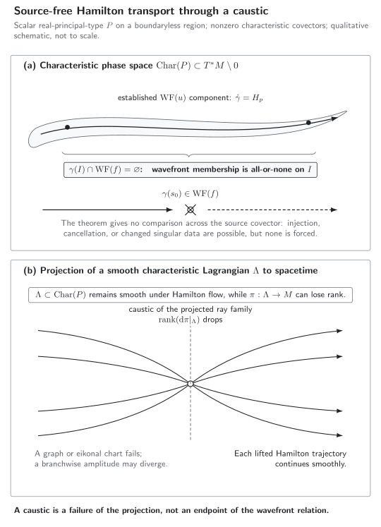
Phase-space transport, rather than a base-space amplitude formula, controls singularities. On a source-free real-principal-type segment, the Hamilton flow of $p$ carries an established wavefront component along $\operatorname{Char}(P)$. For the illustrated focused-ray family, a caustic is a rank loss of $\pi|_\Lambda$: the projected null rays focus, a branchwise Van Vleck or stationary-phase amplitude may diverge, and the lifted bicharacteristics continue. At $\gamma(s_0)\in\operatorname{WF}(f)$ for $Pu=f$, the homogeneous propagation statement no longer determines what crosses. Boundaryless schematic; not to scale. Semantic description (JSON).

The ordinary wavefront set records only smooth versus nonsmooth directions. It does not say that the leading distributional type stays fixed. For each selected geodesic branch, let $\sigma$ denote one-half its signed squared geodesic interval wherever that branch is smooth—typically in a region between successive caustics—and let $\operatorname{PV}$ denote the Cauchy principal value. In specified four-dimensional geometries, comparing these branchwise representations across conjugate points shows a Green-function singularity cycling between $\delta(\sigma)$ and $\operatorname{PV}(1/(\pi\sigma))$, with multiplicity-dependent signs Harte and Drivas 2012, §§ IV–V (Open PDF). This is a leading-singularity and Maslov-phase statement; its overall signs depend on the conventions for $\sigma$ and the Green function. The invariant conclusion used here is only that the lifted wavefront relation continues.

Where the ordinary theorem stops

A source wavefront

If $Pu=f$, membership in $\operatorname{WF}(u)$ is constant on each connected component of a bicharacteristic after removing $\operatorname{WF}(f)$. At a source covector, the theorem makes no comparison between the two sides. A singular source may inject, alter, or cancel singular data in the selected global solution; it need not do any of them. Kernel composition therefore supplies an inclusion rather than guaranteeing that every allowed outgoing branch occurs. But cancellation cannot erase one isolated point of a connected source-free segment and allow the same singularity to reappear later: absence propagates too. Mere membership of the base point in $\operatorname{supp}f$ is insufficient—what matters is the covector-level set $\operatorname{WF}(f)$.

A timelike boundary

An interior null bicharacteristic reaching a boundary does not come with an automatic law of reflection. A concrete replacement theorem is available on $X=M\times\mathbb R_t$ for $P=D_t^2-\Delta_M$, where $M$ is a Riemannian manifold with corners and $u\in H^1_{\mathrm{loc}}$ obeys homogeneous Dirichlet or Neumann conditions. In that model, the $b$-wavefront set records nonsmoothness in covectors dual to vector fields tangent to the boundary, and maximally extended generalized broken bicharacteristics encode interior travel together with reflected or glancing continuation. Corner diffraction is a further regime, and changing the boundary condition can change the returning singularity. See Vasy 2008, Theorems 8.1 and 8.5. Other normally hyperbolic boundary problems require a theorem matched to their operator, boundary geometry, domain, and boundary condition.

A radial set or asymptotic boundary

After compactifying phase space, $H_p$ can become radial at a source or sink: its projected direction on the cosphere bundle degenerates. The ordinary flow-box argument then supplies no useful crossing estimate. Radial-point estimates use one-sided hypotheses and Sobolev thresholds that depend on subprincipal data; they cannot be replaced by the slogan “singularities follow rays.” See Haber and Vasy 2015, § 1 and Theorems 1.4–1.6 (Open PDF).

Systems and gauge fields

For a vector bundle operator with scalar principal symbol $p\,\mathbf1$, the base wavefront still follows the scalar null geometry. The fibre component carries additional information. For systems of real principal type, Dencker’s polarization set and connection transport the allowed polarization along the bicharacteristic Dencker 1982. An unfixed gauge equation may instead have a degenerate principal symbol; one must impose a valid gauge reduction or use a theorem for the constrained complex before invoking scalar propagation.

Regularity is not decay

Wavefront propagation is local in phase space. It does not prove energy or dispersive decay, resolve trapping, locate resonances or quasinormal frequencies, establish scattering or asymptotic completeness, or guarantee geodesic completeness. The constant solution $u=1$ of the massless wave equation already has empty wavefront set and no time decay. Those global questions require energy, resolvent, or scattering estimates beyond this theorem.

Common pitfalls

Including the zero section. Wavefront sets contain nonzero covectors only. Real-principal-type hypotheses and the Klein–Gordon characteristic cone must therefore be stated in $T^*M\setminus0$.

Confusing retarded support with positive frequency. Retarded and advanced describe the causal location of the output base point. A delta front has both conormal signs; the Hadamard condition is what selects one frequency orientation for a two-point function.

Calling the orbit complete. A maximal segment is extended only as far as its source-free microlocal domain permits. Global hyperbolicity gives global Green operators, not null-geodesic completeness.

Assuming every characteristic covector occurs. Propagation constrains a singularity that is present; it does not manufacture one. A smooth compact source produces a smooth Green response, and kernel composition may give a strict inclusion because of cancellation.

Interpreting a divergent WKB amplitude as smoothing. A caustic is a failure of a projected phase chart. The lifted Lagrangian and its wavefront relation can remain smooth while amplitudes and Maslov phases require a different representation.

Stopping after two-slot propagation. Applying the field equation separately in each variable does not exclude partial-zero covectors. The time-slice and kernel-composition step is logically independent.

Exercises

1. Characteristic invariance and symbol rescaling. Show that $H_pp=0$ and that replacing $p$ by $ap$, with $a$ smooth, real, nonvanishing, and degree-zero homogeneous on the conic region, preserves the unparametrized characteristic orbits.

Solution

Antisymmetry of the Poisson bracket gives $H_pp=\{p,p\}=0$, so the flow preserves each level set of $p$. The Leibniz rule gives

$$H_{ap}=aH_p+pH_a.$$

On $p=0$, this reduces to $aH_p$. A nonzero factor changes the speed, and a negative factor reverses orientation, but the unparametrized orbit is unchanged.

2. Klein–Gordon geodesic flow. Starting from $h=g^{ab}k_ak_b/2$, derive Hamilton’s equations and show that a characteristic projection is a null geodesic.

Solution

Differentiation gives

$$\dot x^a=g^{ab}k_b, \qquad \dot k_a=-\frac12\partial_a g^{bc}k_bk_c.$$

Using $\partial_a g^{bc}=-g^{bd}g^{ce}\partial_a g_{de}$ and defining $\Gamma_{eba}:=g_{ec}\Gamma^c{}_{ba}$ by lowering the first Christoffel index gives the intermediate cancellation

$$\begin{aligned} (\nabla_{\dot x}k)_a &=\dot k_a-\Gamma^c{}_{ba}\dot x^b k_c\\ &=\frac12\partial_a g_{de}\dot x^d\dot x^e -\Gamma_{eba}\dot x^b\dot x^e =0. \end{aligned}$$

Metric compatibility then gives $\nabla_{\dot x}\dot x=0$. Since $h$ is conserved and equals zero on the characteristic set,

$$g(\dot x,\dot x)=g^{-1}(k,k)=2h=0.$$

Thus the projection is an affinely parametrized null geodesic.

3. Wavefront of the retarded light-cone front. Away from $r=0$, find the conormal covectors of $\delta(t-r)/(4\pi r)$ and verify that they are characteristic.

Solution

Multiplication by the smooth nonzero factor $1/(4\pi r)$ does not change the wavefront set. The defining function is $F=t-r$, so the conormals are

$$\lambda\,\mathrm dF = \lambda \left( \mathrm dt- \widehat{\mathbf x}\cdot\mathrm d\mathbf x \right), \qquad \lambda\neq0.$$

Their squared norm is $\lambda^2(1-\lvert\widehat{\mathbf x}\rvert^2)=0$. They therefore lie in the characteristic cone, and their raised vectors are tangent to the outgoing null generators.

4. Retarded is not positive frequency. Why does the front in Exercise 3 contain both $\lambda>0$ and $\lambda<0$ although it is supported on the future light cone?

Solution

A delta distribution on a smooth hypersurface has every nonzero multiple of the hypersurface conormal in its wavefront set. The restriction $t>0$ selects which base-space cone is present, while the sign of $\lambda$ records the two fibre orientations. Support direction and frequency orientation are different data.

5. Crossing a singular source. Suppose a bicharacteristic meets $\operatorname{WF}(f)$ only at $s=s_0$. What does propagation say on the two sides, and what does it say across $s_0$?

Solution

Membership in $\operatorname{WF}(u)$ is all-or-none separately on each connected source-free interval $s<s_0$ and $s>s_0$. The theorem gives no comparison across $s_0$. The source can inject, modify, or cancel a branch in the chosen solution, but none of those outcomes follows from propagation alone.

6. Exact null caustic model. For the homogeneous phase in the caustic section, derive the fiber-critical equations. Then verify that its generated covector is null and nonzero at $t=s=0$, while the projection loses rank there.

Solution

Differentiating with respect to the conic fiber variables gives

$$\begin{aligned} 0=\partial_\mu\Phi &=x-\frac{t\mu}{\sqrt{\mu^2+\lambda^2}} -\frac{\mu^2}{\lambda^2},\\ 0=\partial_\lambda\Phi &=z-\frac{t\lambda}{\sqrt{\mu^2+\lambda^2}} +\frac{2\mu^3}{3\lambda^3}. \end{aligned}$$

Setting $s=\mu/\lambda$ yields the displayed base map $q(t,s)$ and

$$k=\mathrm d_{t,x,z}\Phi =\lambda\left(-\sqrt{1+s^2},s,1\right).$$

Therefore $k_t^2-k_x^2-k_z^2=0$. At $s=0$, $k=\lambda(-1,0,1)\neq0$. Meanwhile

$$\left.\partial_tq\right|_{0,0}=(1,0,1), \qquad \left.\partial_sq\right|_{0,0}=0,$$

so the generic rank-two family projection drops to rank one. The lift remains smooth because $\partial_s k|_{s=0}=(0,\lambda,0)$ is nonzero and independent of the radial $\lambda$ direction.

7. Diagonal cancellation in the causal propagator. Let $(x,k;x,k)\in\Delta^*$ with $p(x,k)\neq0$. Explain why the common local inverse singularity of $G_{\mathrm{ret}}$ and $G_{\mathrm{adv}}$ cancels in $E=G_{\mathrm{ret}}-G_{\mathrm{adv}}$. Why can characteristic diagonal pairs remain?

Solution

Near a noncharacteristic covector, $P$ is elliptic. Its microlocal inverse symbol is unique modulo a smoothing term, so the retarded and advanced support choices have the same diagonal singularity there. Their difference is therefore smooth near $(x,k;x,k)$ when $p(x,k)\neq0$.

At a characteristic covector, elliptic uniqueness no longer applies. The retarded and advanced kernels carry different future and past Hamilton flow-outs, and their null diagonal directions are the meeting points of those relations. Hence the noncharacteristic part of $\Delta^*$ cancels from $E$, while the characteristic diagonal remains inside $\mathcal C$.

8. Regularity is not decay. Give a smooth homogeneous solution of the massless wave equation that does not decay in time.

Solution

Take $u=1$. Then $\Box_g u=0$ on any spacetime, $\operatorname{WF}(u)=\varnothing$, and $u$ is constant rather than decaying. Empty wavefront set proves smoothness only; a decay statement needs additional global estimates and hypotheses.

Where this result is used next

Higher-point microlocal spectrum conditions use Hamilton transport on graph-labeled covectors. Hadamard states and the wavefront-set characterization turns the two-point singularity relation into the theorem-level state criterion. The physical propagation of the Hadamard property supplies the complete Cauchy-band and partial-zero argument, while Hadamard admissibility and the two-point wavefront criterion explains the oriented cone’s physical meaning.

References

• Dencker, Nils. “On the Propagation of Polarization Sets for Systems of Real Principal Type.” Journal of Functional Analysis 46, no. 3 (1982): 351–372. DOI.
• Duistermaat, J. J., and Lars Hörmander. “Fourier Integral Operators. II.” Acta Mathematica 128 (1972): 183–269. DOI.
• Fewster, Christopher J. “Polarisation Sets of Green Operators for Normally Hyperbolic Equations.” arXiv:2503.12544v2 (2026). Preprint PDF.
• Haber, Nick, and András Vasy. “Propagation of Singularities around a Lagrangian Submanifold of Radial Points.” Bulletin de la Société Mathématique de France 143, no. 4 (2015): 679–726. DOI and Open PDF.
• Harte, Abraham I., and Theodore D. Drivas. “Caustics and Wave Propagation in Curved Spacetimes.” Physical Review D 85, no. 12 (2012): 124039. DOI. Open PDF.
• Radzikowski, Marek J. “Micro-Local Approach to the Hadamard Condition in Quantum Field Theory on Curved Space-Time.” Communications in Mathematical Physics 179 (1996): 529–553. DOI.
• Vasy, András. “Propagation of Singularities for the Wave Equation on Manifolds with Corners.” Annals of Mathematics 168, no. 3 (2008): 749–812. DOI. Open preprint.