BV–BFV Boundaries, Corners, and Gluing

BV–BFV theory records what the BV master equation becomes when spacetime has a boundary. The boundary term in the variation is promoted to a degree-zero symplectic phase space and cohomological charge; corners continue the construction at higher degree; polarizations and residual fields turn it into a perturbative state; and gluing is a pairing followed by BV pushforward. Each step has its own regularity and anomaly conditions. A successful topological example does not by itself establish bounded four-dimensional gauge theory.

Helpful background. Field variations and boundary terms supplies the variational source of the BFV primitive. Edge modes, subregions, and factorization gives the physical regional problem. State spaces, cobordisms, and gluing gives the functorial comparison.

Enter this chapter

For a compact oriented $d$-manifold $M$, the central compatibility equation is

$$\iota_{Q_M}\omega_M =(-1)^d\delta S_M+\pi_M^*\alpha^\partial_{\partial M}.$$

The bulk BV form has degree $-1$; the induced boundary form $\omega^\partial=\pm\delta\alpha^\partial$ has degree zero. The restriction map intertwines the bulk and boundary cohomological vector fields. This is not a closed-manifold classical master equation with an ignored surface term: another contraction identifies the defect with the BFV charge.

Before using a gluing formula, name the bulk and boundary field complexes, the admissible boundary condition or polarization, the residual cohomology, the measure or half-density, the BFV operator, the corner data, and the weak equivalence under which gauge-fixing changes are compared. In infinite-dimensional field theory, a BV integral denotes a formal perturbative expansion unless a separate measure theorem is supplied.

The dependency diagram follows the one-way construction. The main row starts with the variational defect, derives boundary phase space and charge, selects admissible boundary and residual data, and reaches a relative quantum state and gluing only after anomaly and regularity tests. The lower branch separates AKSZ, edge-mode, and stratified-factorization structures that use the common boundary geometry for different purposes.

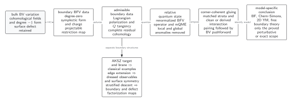
The boundary primitive is derived from the bulk variation. Its symplectic reduction and charge must be compatible before a Lagrangian boundary condition, polarization, or state is selected. Residual cohomology, the modified quantum master equation, anomaly cancellation, corner coherence, and clean BV pushforward then license gluing in the proved model. AKSZ targets, edge extensions, and stratified factorization observables are conditional branches rather than automatic consequences. Every arrow is one-way; the diagram is schematic and not to scale. Structured description and source data (JSON)

The chapter sequence

Read the pages in this order.

1. BV–BFV structures, boundaries, and gluing derives the boundary primitive and verifies the relative equation for Abelian BF theory.
2. Boundary phase spaces, constraints, and the BFV charge constructs first-order Yang–Mills boundary data and separates gauge reduction from charged surface motion.
3. Bulk–boundary master equations and anomaly inflow distinguishes local descent, perturbative QME restoration, and global gauge invariance.
4. Corners, stratification, and higher-codimension data iterates the symplectic hierarchy and tests associativity under face gluing.
5. Gluing, reduction, and composition theorems gives the classical fiber product and quantum pairing-plus-pushforward formula.
6. Edge modes and extended observables at gauge boundaries constructs a dressed Wilson line and diagnoses overcounting and undercounting.
7. AKSZ sigma models as BV–BFV examples transgresses graded Hamiltonian target data and derives admissible branes.
8. Factorization algebras with boundaries and defects replaces bulk Weiss descent by a stratified local-to-global condition.
9. Perturbative boundary gauge theory: scope and open problems compares theorems for BF, Chern–Simons, 2D Yang–Mills, free boundary systems, and Lorentzian Abelian gauge theory.

This order keeps the logical dependencies visible. A boundary state is not defined before the boundary phase space; gluing is not defined before the polarization and residual sector; and a current research construction is not promoted beyond its field content, geometry, perturbative order, or limiting assumptions.

Hypotheses and licensed conclusions

Domains, required hypotheses, directional results, and failure tests for BV–BFV boundaries and gluing

Object and domain	Required hypotheses	Licensed result	Excluded converse or upgrade	Adversarial check
Bulk BV theory on $M$ with boundary	Projectable $Q_M$; surjective boundary restriction; exact or prequantum boundary form; controlled variational signs and domains	Boundary BFV phase space, charge, and modified classical master equation	A closed-manifold CME cannot be used after discarding the surface term	Vary the action and retain every integration-by-parts contribution
Boundary constraint system	Regular coisotropic zero locus; declared gauge subgroup; smooth or derived reduction; integrable generators	BFV resolution and reduced boundary observables	A transformation with nonzero surface charge is not automatically gauge	Quotient a Maxwell flux sector by arbitrary boundary parameters and count the lost directions
Boundary condition or polarization	Lagrangianity; $Q^\partial$ tangency; compatible primitive; finite or controlled intersection with evolution relation	Admissible boundary problem and state-space polarization	Dirichlet-looking constraints need not cancel symplectic flux	Evaluate the boundary Green form on allowed variations
Manifold with corners	Iterated restriction; shifted symplectic degrees; compatible corner charges and endpoint polarizations; refinement coherence	Extended BV–BFV data and associative face composition in the proved model	Codimension-one compatibility does not erase corner terms	Compare two orders of gluing three faces
Perturbative quantum state	Gauge fixing; finite residual sector; renormalized BFV operator; local and global anomaly cancellation; mQME	Cohomology class of a formal boundary state	No convergent measure, positivity, or global vacuum follows from a formal QME	Retain a nonzero anomaly class or determinant-line holonomy
Cut $M=M_1\cup_\Sigma M_2$	Clean or derived intersection; complementary polarizations; matching corner data; one copy of each residual mode; BV pushforward	Paired state satisfying the mQME and composition up to the declared equivalence	Multiplication followed by an unspecified functional integral is not a gluing theorem	Double-count a harmonic mode and compare determinant degrees
Boundary model or extrapolation	Named BF, Chern–Simons, 2D Yang–Mills, free stratified, or smoothened Abelian theorem with its geometry and order	Exactly the model-specific classical, perturbative, or gluing statement proved	No general four-dimensional non-Abelian continuum existence or positivity theorem follows	Replace a Gaussian BF cylinder by 4D Yang–Mills and list every missing analytic input

Structured table data (JSON) preserves the caption, scoped headers, rows, and reading order.

The failure map identifies the first lost conclusion when a hypothesis is removed. Its purpose is not to declare the entire theory invalid: a bulk classical complex may survive after a boundary condition fails, and a local Ward identity may survive after global anomaly cancellation fails.

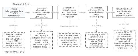
Each dashed branch removes one concrete input. Ignoring the variational defect restores neither the closed CME nor a boundary charge; an incompatible boundary subspace leaves symplectic flux; omitted zero modes and corner pairings spoil cut independence or associativity; local anomaly cancellation can leave global holonomy; and a valid BF or 2D Yang–Mills gluing formula cannot be promoted to 4D non-Abelian Yang–Mills without renormalized boundary observables, regulator removal, and positivity. The diagram is schematic and not to scale. Structured description and source data (JSON)

Scope and current boundary

The classical framework and its regular gluing relations are developed in Cattaneo, Mnev, and Reshetikhin 2014, §§3–7, pp. 8–54. Their perturbative quantum construction supplies states, residual fields, the mQME, and gluing for Abelian BF and specified BF-like models Cattaneo, Mnev, and Reshetikhin 2018, §§2–4, pp. 8–61. Corners are explicit in two-dimensional Yang–Mills Iraso and Mnev 2019, §§4.1–4.7, pp. 35–60, and stratified quantum observables are proved for a class of free theories topological normal to the boundary Gwilliam, Rabinovich, and Williams 2021, Theorems 4.1–4.2.

As of July 2026, smoothened-boundary pAQFT gives a renormalized Lorentzian BV–BFV construction and an Abelian Yang–Mills causal-cylinder example, with the sharp-boundary theorem conditioned on convergence of the smoothing limit Rejzner and Schiavina 2026, §§4–5 and Theorem 5.8. This is a significant bridge, but it does not settle arbitrary corners, non-Abelian 4D regulator removal, or a positive nonperturbative Hilbert space.

Review the chapter

Before accepting a boundary or gluing claim, answer the following.

1. Which bulk fields, boundary traces, symplectic forms, primitives, and $Q$ maps occur?
2. Does the stated master equation include the boundary BFV charge with consistent signs?
3. Which boundary transformations are gauge and which carry Hamiltonian charge?
4. Is the boundary condition Lagrangian and preserved by the boundary differential?
5. Which cohomology classes are residual fields, and where are they integrated?
6. Which face, corner, and endpoint data make repeated gluing coherent?
7. Is the boundary state a function, half-density, formal series, or operator-algebraic state?
8. Which local and global anomaly classes have been tested?
9. Does the gluing theorem use an ordinary, clean, or derived fiber product?
10. Which theorem supports the claimed dimension, gauge group, loop order, and continuum status?

Synthesis exercise

A perturbative Abelian BF state satisfies the mQME and glues across a circle after residual-field reduction. May its formula be used unchanged for non-Abelian four-dimensional Yang–Mills on a box?

Solution

No. The Abelian BF nonzero-mode integral is Gaussian and its residual sector is de Rham cohomology. Four-dimensional non-Abelian Yang–Mills needs interacting bulk, boundary, and corner renormalization; a proper global gauge complex; anomaly cancellation; compatible polarizations; infrared control; regulator removal; and positivity or reconstruction. The BF formula supplies a structural model for pairing and BV pushforward, not the missing analytic theorem.

References

• Cattaneo, Alberto S., Pavel Mnev, and Nicolai Reshetikhin. “Classical BV Theories on Manifolds with Boundary.” Communications in Mathematical Physics 332 (2014): 535–603. DOI; Open PDF.
• Cattaneo, Alberto S., Pavel Mnev, and Nicolai Reshetikhin. “Perturbative Quantum Gauge Theories on Manifolds with Boundary.” Communications in Mathematical Physics 357 (2018): 631–730. DOI; Open PDF.
• Gwilliam, Owen, Eugene Rabinovich, and Brian R. Williams. “Factorization Algebras and Abelian CS/WZW-Type Correspondences.” 2021. arXiv:2001.07888.
• Iraso, Riccardo, and Pavel Mnev. “Two-Dimensional Yang–Mills Theory on Surfaces with Corners in Batalin–Vilkovisky Formalism.” Communications in Mathematical Physics 370 (2019): 637–702. DOI; Open PDF.
• Rejzner, Katarzyna, and Michele Schiavina. “Perturbative Algebraic Quantum Field Theory with Smoothened Boundary.” 2026. arXiv:2607.13765.