Higher-Point Microlocal Spectrum Conditions

The microlocal spectrum condition, or $\mu$SC, is the curved-spacetime replacement for a joint energy–momentum support condition. It does not assign a globally conserved momentum to each spacetime point. Instead, it asks whether every singular covector tuple of every $n$-point distribution can be assembled from future-directed causal covectors transported along the edges of a finite graph. The graph remembers the frequency orientation that singular support forgets, while its incidence rule supplies exactly the closure properties needed for products, Wick contractions, and changes of state within a folium.

One distinction is essential from the start: in the original smooth $\mu$SC, an edge follows a piecewise-smooth path, which need not be causal, while its parallel covector label is future causal. Requiring the path itself to be causal or null defines a stronger variant.

Required background. Microlocal calculus for quantum fields supplies wavefront cones and their orientation; propagation of singularities for hyperbolic fields supplies parallel transport along null Hamilton flow.

Helpful background. Wightman functions and spectral support gives the Minkowski antecedent; wavefront-set products, pullbacks, and pushforwards supplies the product calculus used below.

From spectral support to graph cones

Let $M$ be a time-oriented Lorentzian spacetime with Levi–Civita connection. For a scalar field state $\omega$ on the Borchers–Uhlmann algebra, write

$$\omega_n(f_1\otimes\cdots\otimes f_n) = \omega\!\left(\phi(f_1)\cdots\phi(f_n)\right)$$

for its ordered $n$-point distributions. The indices $1,\ldots,n$ record field-argument order, not chronological or causal order.

At a base point $x=(x_1,\ldots,x_n)\in M^n$, choose a finite multigraph with edge-copy set $E$ on the ordered vertices $1,\ldots,n$. Parallel edges are allowed and may follow different immersed paths. For each $e\in E$, use one representative and write its source and target as $s(e)<t(e)$:

1. the edge is oriented $s(e)\to t(e)$;
2. it is immersed as a piecewise-smooth path $\gamma_e$ from $x_{s(e)}$ to $x_{t(e)}$;
3. it carries a covariantly constant future-directed causal covector field $\xi_e$ along $\gamma_e$.

The zero covector is allowed as an edge label. This is useful when an external tensor product leaves some slots smooth. At vertex $i$, take the signed incidence sum

$$k_i = \sum_{e:\,s(e)=i}\xi_e(x_i) - \sum_{e:\,t(e)=i}\xi_e(x_i).$$

Only edges that are present contribute. This one-representative convention is equivalent to the original doubled convention: every oriented edge $e$ is accompanied by $e^{-1}$, the reverse edge carries $-\xi_e$, and one sums all labels whose source is vertex $i$.

The smooth-path graph cone $\Gamma_n$ is the union of all tuples

$$(x_1,k_1;\ldots;x_n,k_n)\in T^*M^n\setminus0$$

obtained in this way. The total zero covector is excluded because a wavefront set never contains it, but individual slots $k_i=0$ are permitted. The state satisfies $\mu$SC when

$$\operatorname{WF}(\omega_n)\subset\Gamma_n \qquad\text{for every }n\geq1.$$

This is Brunetti, Fredenhagen, and Köhler 1996, Definition 4.1 and footnote 2, preprint pp. 9–10 (Open PDF). All displayed fiber signs use the site’s forward Fourier phase $e^{+ip\cdot x}$. Brunetti, Fredenhagen, and Köhler define wavefront directions with the opposite Fourier kernel; when their Fourier-fiber variables enter the flat-space reduction below, they are reflected as explained on the prerequisite microlocal-calculus page. The chapter comparison table places this condition beside the product, propagation, Hadamard, and renormalization hypotheses it does—and does not—supply.

Why the first nonzero slot points to the future

Let $i_0$ be the smallest index for which $k_{i_0}\neq0$. At vertex $1$, the balance contains only future-causal outgoing labels. If it vanishes, every such edge-copy label vanishes because the closed future cone is pointed. Repeating the argument at vertices $2,\ldots,i_0-1$ shows that all labels arriving at $i_0$ from earlier vertices are zero. Consequently,

$$k_{i_0}=\sum_{e:\,s(e)=i_0}\xi_e(x_{i_0})$$

is a nonzero future-directed causal covector. In particular,

$$\Gamma_n\cap(-\Gamma_n)=\varnothing.$$

This small lemma is the engine behind the product theorem and the edge-reversal test below. Notice that it compares covectors in a single fiber at each step. On a generic curved spacetime, the expression $\sum_i k_i$ is meaningless because the $k_i$ live in different cotangent spaces.

Smooth, causal-path, null-path, and analytic variants

It helps to put the variants in order. Let $\Gamma_n^{\mathrm{sm}}$ denote the cone just defined, $\Gamma_n^{\mathrm{c}}$ the cone obtained by requiring every path $\gamma_{ij}$ to be causal, and $\Gamma_n^{\mathrm{ll}}$ the cone obtained by requiring null paths. Then

$$\Gamma_n^{\mathrm{ll}} \subseteq \Gamma_n^{\mathrm{c}} \subseteq \Gamma_n^{\mathrm{sm}}.$$

Therefore a wavefront inclusion into $\Gamma_n^{\mathrm{ll}}$ is the strongest of these three requirements. The ordinary Minkowski spectrum condition implies the original smooth-path $\mu$SC, but that proof does not automatically establish either stronger path restriction; the distinction is explicit in Brunetti, Fredenhagen, and Köhler 1996, Theorem 4.6 and the discussion after it, preprint pp. 13–14 (Open PDF).

The analytic microlocal spectrum condition is a different strengthening. On a real-analytic spacetime it replaces the smooth wavefront set by the analytic wavefront set $\operatorname{WF}_{\!A}$; it is not merely another choice of edge path. It implies the Reeh–Schlieder property under the state and GNS hypotheses of Strohmaier, Verch, and Wollenberg 2002, Theorem 5.4 and Corollary 5.5 (Open PDF). Their Theorem 6.3 proves ordinary $\mu$SC for quasifree Klein–Gordon ground and KMS states on a globally hyperbolic stationary spacetime; the analytic conclusion additionally requires the spacetime and its stationary flow to be real analytic.

For a quasifree Klein–Gordon state on a globally hyperbolic spacetime, the smooth $\mu$SC hierarchy is equivalent to the Hadamard condition on its two-point function Strohmaier, Verch, and Wollenberg 2002, Proposition 6.1 (Open PDF). The Klein–Gordon field equation, canonical commutator, positivity, and state hypotheses are part of that statement. The next page proves the two-point characterization itself; the present page explains how its orientation propagates through the hierarchy.

Why the graph calculus is stable

The graph definition is designed so that several operations become almost visible.

Addition and pointwise products

At a fixed base point, take the disjoint union of two realizing multigraphs, retaining every parallel edge and its own immersed path. The vertex balances then add. Only edge copies with the identical immersed path may optionally be combined by adding their parallel labels; the future cone’s convexity preserves future causality. Thus

$$\Gamma_n\oplus\Gamma_n\subset\Gamma_n.$$

Together with $\Gamma_n\cap(-\Gamma_n)=\varnothing$, Hörmander’s criterion shows that two distributions $u,v$ with wavefront sets in $\Gamma_n$ have a well-defined pointwise product. Moreover,

$$\operatorname{WF}(uv) \subset \operatorname{WF}(u) \cup \operatorname{WF}(v) \cup \bigl(\operatorname{WF}(u)\oplus\operatorname{WF}(v)\bigr) \subset\Gamma_n.$$

Brunetti, Fredenhagen, and Köhler use precisely these facts to prove closure of $\mu$SC states under their pointwise product construction and stability throughout the corresponding folium Brunetti, Fredenhagen, and Köhler 1996, Lemma 4.2 and Theorems 4.4–4.5, preprint pp. 10–13 (Open PDF). The cone calculation licenses the distributions; positivity of a functional remains a separate algebraic statement.

Tensor factors and partial-zero slots

If a distribution depends singularly only on variables in a block $B\subset\{1,\ldots,n\}$, its exterior extension to $M^n$ has zero covectors in the other slots. A realizing graph simply has no nonzero edges incident on those vertices. This is why partial-zero slots must remain in $\Gamma_n$: they occur in every Wick contraction before the factors are combined.

The same observation makes the cone family compatible with disjoint unions and with order-preserving interleavings of blocks—that is, permutations which preserve the inherited order inside every block. Arbitrary permutations need not preserve $\Gamma_n$. This restricted compatibility underlies the equivalence between formulating $\mu$SC for full $n$-point functions and for truncated, or connected, functions Sanders 2010, Proposition 2.5(3) and Lemma 2.6 (Open PDF).

Differential equations and differentiated fields

The graph condition does not imply a field equation. If, separately, a free Klein–Gordon hierarchy obeys

$$P_i\omega_n=0$$

in the $i$th variable, microlocal elliptic regularity says that every wavefront tuple with $k_i\neq0$ has $k_i$ in the characteristic set of $P$. For a normally hyperbolic Klein–Gordon operator, that means $k_i$ is null. Conversely, applying any differential operator to an $n$-point distribution cannot enlarge its wavefront set:

$$\operatorname{WF}(D\omega_n)\subseteq\operatorname{WF}(\omega_n).$$

Thus the field equation sharpens the vertex tuple: every nonzero external covector $k_i$ must be characteristic. It does not force every internal edge label of every realizing graph to be null; timelike labels may split or cancel at a vertex. Differentiated field insertions preserve an existing wavefront bound, but neither conclusion comes from $\mu$SC alone.

The flat-space spectrum condition builds a chain

Minkowski space is special because translation identifies all cotangent fibers. With the site’s Fourier phase $e^{+ip\cdot x}$, translation invariance and the ordinary Wightman spectrum condition give, for a momentum-space wavefront tuple,

$$\sum_{i=1}^{n}p_i=0, \qquad S_j:=\sum_{i=1}^{j}p_i\in\overline V_+, \qquad 1\leq j<n.$$

Now draw the chain

$$1\longrightarrow2\longrightarrow\cdots\longrightarrow n$$

immerse each edge as the straight segment from $x_j$ to $x_{j+1}$—the segment need not be causal—and give it the constant future-causal label $S_j$. Its signed vertex balances are

$$p_1=S_1, \qquad p_j=S_j-S_{j-1}\quad(2\leq j<n), \qquad p_n=-S_{n-1}.$$

The chain therefore realizes the original momentum tuple in $\Gamma_n$. This is the substantive reduction from the ordinary spectrum condition to $\mu$SC, not merely the identity $\sum_i p_i=0$ Brunetti, Fredenhagen, and Köhler 1996, Theorem 4.6 (Open PDF). The displayed $p_i$ and $S_j$ already use the site’s $e^{+ip\cdot x}$ convention, with the source’s opposite Fourier-fiber labels reflected. On a curved spacetime there is no canonical analogue of the total sum; parallel-transported edge data replace it.

Quasifree Hadamard hierarchies

Let $\omega$ be a centered quasifree scalar state. Its odd $n$-point distributions vanish, while Wick’s theorem gives

$$\omega_{2r}(x_1,\ldots,x_{2r}) = \sum_{P\in\operatorname{Pair}(2r)} \prod_{\{i,j\}\in P}\omega_2(x_i,x_j).$$

Each two-point factor is pulled back from $M^2$ to the slots $i,j$ of $M^{2r}$, so its wavefront tuples have zero covectors in all other slots. For a Hadamard two-point function,

$$\operatorname{WF}(\omega_2) = \left\{ (x,k;x',-k'): (x,k)\sim(x',k'),\ k\in\overline V_+\setminus0 \right\},$$

where $\sim$ denotes cotangent transport along the relevant null geodesic. Radzikowski’s theorem identifies this oriented relation with the local Hadamard form under the free-field hypotheses Radzikowski 1996, Theorem 5.1.

For one pairing $P$, draw one lower-to-higher edge for every pair $\{i,j\}$. The pulled-back factor supplies its future null label. Since the pairs are disjoint, their product is an exterior tensor product in disjoint variables, and summing its slot covectors gives exactly the incidence tuple of that pairing graph. A smooth factor is represented by a zero label. Finally, the wavefront set of a finite sum lies in the union of the summands’ wavefront sets. Hence

$$\operatorname{WF}(\omega_{2r})\subset\Gamma_{2r}, \qquad \operatorname{WF}(\omega_{2r+1})=\varnothing.$$

This proves the quasifree hierarchy result Brunetti, Fredenhagen, and Köhler 1996, Proposition 4.3 (Open PDF). A nonzero smooth one-point function adds only smooth factors and does not alter the bound.

The four-point calculation

Wick’s theorem gives three terms:

$$\omega_4 = \omega_2(x_1,x_2)\omega_2(x_3,x_4) + \omega_2(x_1,x_3)\omega_2(x_2,x_4) + \omega_2(x_1,x_4)\omega_2(x_2,x_3).$$

For the middle term, let the edges $1\to3$ and $2\to4$ carry future null covectors $a$ and $b$, with $a\neq0$. Write $a_1,a_3$ and $b_2,b_4$ for their values at the two endpoints after parallel transport. The vertex tuple is

$$(k_1,k_2,k_3,k_4) = (a_1,b_2,-a_3,-b_4)\in\Gamma_4.$$

The other two Wick terms give the other two pairing graphs. The figure makes the distinction between base-point pairing and covector orientation explicit; inspect the sign at the earliest nonzero vertex.

On a narrow screen, swipe or use the Left and Right arrow keys to pan across the figure. Home and End move to its edges. A full-size link is also available.

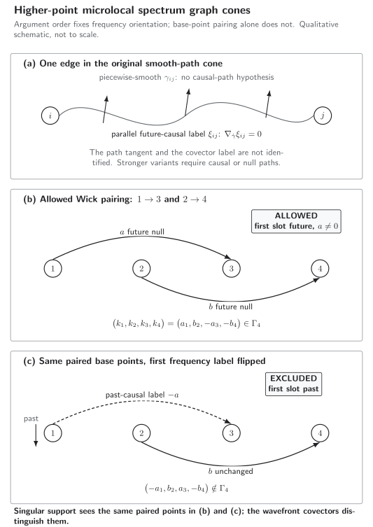
The smooth $\mu$SC constrains a parallel future-causal edge label, not the tangent of its piecewise-smooth path. For $a\neq0$, a quasifree $1\to3$, $2\to4$ contraction produces $(a_1,b_2,-a_3,-b_4)\in\Gamma_4$. Keep the first graph representative directed $1\to3$ but flip only its covector label from $a$ to the past-causal $-a$. The paired base points are unchanged, while the tuple becomes $(-a_1,b_2,a_3,-b_4)$; its first nonzero slot is past directed, so it cannot lie in $\Gamma_4$. Original schematic; not to scale. Semantic description and exact sign data (JSON).

This is the higher-point construction used by the physical Hadamard admissibility criterion. Here the theorem-level work is the graph-cone bound; the physical volume owns state selection and interpretation.

Full and truncated functions

Write $\omega_n^T$ for the truncated distributions. The moment–cumulant relation is

$$\omega_n(x_1,\ldots,x_n) = \sum_{\mathcal P\in\operatorname{Part}(n)} \prod_{B\in\mathcal P}\omega^T_{|B|}(x_B).$$

Every block $B$ is evaluated in increasing argument order and occupies disjoint variable slots. Because the graph cones are stable under disjoint block unions and order-preserving interleavings—not arbitrary permutations—$\mu$SC for all full distributions is equivalent to $\mu$SC for all truncated distributions; one direction uses the partition formula and the other its Möbius inversion Sanders 2010, Proposition 2.5(3) and Lemma 2.6 (Open PDF).

For a quasifree state, $\omega_n^T=0$ for $n\neq2$, which reduces everything to pairings. More generally, Sanders proves that a generalized Hadamard state with scalar, or c-number, commutation relations has smooth $\omega_n^T$ for $n\neq2$ and therefore satisfies the smooth-path $\mu$SC. Here

$$\omega_{2-}:=\frac{1}{2}\!\left(\omega_2-\omega_2^{\mathrm{op}}\right), \qquad \omega_2^{\mathrm{op}}(x_1,x_2):=\omega_2(x_2,x_1),$$

is the antisymmetric part of the two-point distribution and is proportional to the c-number commutator. The causal- and null-path conclusions additionally require $\operatorname{WF}(\omega_{2-})\subset\Gamma_2^{\mathrm c}$ and $\operatorname{WF}(\omega_{2-})\subset\Gamma_2^{\mathrm{ll}}$, respectively Sanders 2010, Theorem 4.2 and Corollary 4.3 (Open PDF). Without such a theorem, an admissible two-point function does not determine or control arbitrary connected three- and higher-point singularities.

The decisive edge-reversal test

Return to the middle four-point pairing and assume $a\neq0$. Keep the same base paths between $x_1,x_3$ and $x_2,x_4$, but reverse the frequency label on the first pair. The candidate tuple becomes

$$(-a_1,b_2,a_3,-b_4).$$

Its first slot is nonzero and past directed. The first-nonzero-slot lemma therefore rules it out of $\Gamma_4$. Yet the projection to base points—the information retained by singular support—is unchanged. Thus a symmetric statement such as “singularities occur only when the points are joined by admissible paths” is too weak: it cannot distinguish the allowed Wick contraction from its wrong-frequency counterpart.

The test also shows why “reverse any edge” is not a sufficient argument. One must identify a reversal that makes the globally earliest nonzero slot past directed, as the $1\to3$ reversal does here.

What the condition does not prove

$\mu$SC is an upper bound on possible singular directions. It does not require every allowed direction to occur. Checking the cone inclusions for a candidate hierarchy does not by itself establish that the hierarchy is a positive state, and it does not supply the field equation, commutator, locality, normalization, stationarity, a preferred vacuum, uniqueness, or state existence. Those are separate hypotheses or constructions.

Likewise, the smooth-path condition should not be silently upgraded to the causal-path, null-path, or analytic version. Every stronger conclusion must name the additional spacetime, field, state, and regularity assumptions that license it.

Common pitfalls

Making the graph path causal by definition. The original $\Gamma_n$ requires a piecewise-smooth path carrying a parallel future-causal covector. Causal and null paths define smaller cones and stronger conditions.

Adding covectors from different points. The vertex balance is fiberwise. A total momentum sum is canonical in Minkowski space after translation identifies the fibers, not on a general curved spacetime.

Discarding partial-zero slots. Exterior tensor products and Wick factors naturally produce wavefront tuples with smooth spectator variables. Only the total zero tuple is excluded.

Treating a two-point bound as a general reconstruction theorem. Wick factorization, scalar commutation relations, or another higher-point theorem is needed. A nonquasifree hierarchy may contain independent connected singularities.

Exercises

1. The two-point cone. Use the one-edge graph to describe $\Gamma_2$. Under the Klein–Gordon equation, what further restriction appears, and what is still needed to obtain the full Hadamard relation?

Solution

For an edge $1\to2$ carrying a future-causal parallel covector $a$, the vertex tuple is $(a_1,-a_2)$. Thus the first nonzero slot is future directed and the second is its transported negative. If $P_1\omega_2=P_2\omega_2=0$, microlocal elliptic regularity forces each nonzero endpoint covector to be characteristic, hence null for Klein–Gordon. Endpoint nullness alone does not show that the two covectors lie on the same null bicharacteristic. Propagation of singularities for the bisolution supplies that transport, while the fixed commutator supplies both branches needed to identify the full singular relation. Together with positivity, the state hypotheses, and global hyperbolicity, this yields the Hadamard equality; cone inclusion alone is insufficient.

2. Cone addition and the product criterion. Show directly that the sum of two graph tuples at the same base point is again a graph tuple. Why can the sum never be the total zero tuple?

Solution

Take the disjoint union of the two realizing multigraphs, retaining parallel edges separately when their immersed paths differ. The new vertex balances are the sums of the old balances. Edge copies on the identical path may instead be combined: the sum of their parallel future-causal labels is again parallel and future causal. If the total tuple vanished, choose the smallest vertex incident on a nonzero label. Its balance would be a nonzero sum of future-causal covectors and could not vanish. Therefore $\Gamma_n\oplus\Gamma_n\subset\Gamma_n$ and $\Gamma_n\cap(-\Gamma_n)=\varnothing$; Hörmander’s no-opposite-covector criterion then licenses the product.

3. Build the Minkowski chain. Suppose $\sum_i p_i=0$ and every prefix $S_j=\sum_{i=1}^j p_i$ lies in $\overline V_+$. Verify that a chain with edge $j\to j+1$ labeled by $S_j$ has vertex balances $p_i$.

Solution

Vertex $1$ has only the outgoing label $S_1=p_1$. An interior vertex $j$ has outgoing label $S_j$ and incoming label $S_{j-1}$, so its balance is $S_j-S_{j-1}=p_j$. Vertex $n$ has only the incoming label $S_{n-1}$, hence balance $-S_{n-1}=p_n$ by total momentum conservation. Every edge label is future causal, so the tuple lies in $\Gamma_n$.

4. Enumerate the four-point pairings. Write the graph and vertex tuple for each of the three terms in the centered quasifree four-point function.

Solution

For $\omega_{12}\omega_{34}$, use edges $1\to2$ and $3\to4$, giving $(a_1,-a_2,b_3,-b_4)$. For $\omega_{13}\omega_{24}$, use $1\to3$ and $2\to4$, giving $(a_1,b_2,-a_3,-b_4)$. For $\omega_{14}\omega_{23}$, use $1\to4$ and $2\to3$, giving $(a_1,b_2,-b_3,-a_4)$. In each formula the repeated letter denotes one parallel-transported edge label, not an identification of different cotangent fibers.

5. Add the field equation. Let $P$ be normally hyperbolic and suppose $P_i\omega_n=0$. Prove that a wavefront tuple cannot have a timelike or spacelike nonzero covector in slot $i$.

Solution

Microlocal elliptic regularity gives $\operatorname{WF}(\omega_n)\subset\operatorname{Char}(P_i)$ in every slot where the covector is nonzero. The principal symbol of a normally hyperbolic operator is $g^{-1}(k_i,k_i)$ up to a nonzero sign. Its characteristic set is therefore $g^{-1}(k_i,k_i)=0$ with $k_i\neq0$. Timelike and spacelike nonzero covectors are excluded. A zero slot remains possible because it represents smooth dependence on that variable within the selected wavefront tuple.

6. Perform the adversarial reversal. In the $1\to3$, $2\to4$ pairing, flip the sign of the first edge label only. Explain both why the result is excluded and why singular support cannot detect the change.

Solution

The allowed tuple $(a_1,b_2,-a_3,-b_4)$ becomes $(-a_1,b_2,a_3,-b_4)$. Since $a\neq0$, slot $1$ is the earliest nonzero slot and is past directed, contradicting the necessary first-nonzero-slot property of $\Gamma_4$. The endpoints and paths of both pairs are unchanged, so projecting the two covector configurations to $M^4$ gives the same base-point singular set. Singular support retains that projection and loses the sign that distinguishes them.

Continue the microlocal chain

Next, Hadamard states and the wavefront-set characterization proves when the oriented two-point relation is equivalent to the local Hadamard expansion. Then Wick polynomials under microlocal conditions uses that control to license coincident composite fields.

References

• Brunetti, Romeo, Klaus Fredenhagen, and Michael Köhler. “The Microlocal Spectrum Condition and Wick Polynomials of Free Fields on Curved Spacetimes.” Communications in Mathematical Physics 180 (1996): 633–652. DOI. Open PDF.
• Radzikowski, Marek J. “Micro-Local Approach to the Hadamard Condition in Quantum Field Theory on Curved Space-Time.” Communications in Mathematical Physics 179 (1996): 529–553. DOI.
• Sanders, Ko. “Equivalence of the (Generalised) Hadamard and Microlocal Spectrum Condition for (Generalised) Free Fields in Curved Spacetime.” Communications in Mathematical Physics 295 (2010): 485–501. DOI. Open PDF.
• Strohmaier, Alexander, Rainer Verch, and Manfred Wollenberg. “Microlocal Analysis of Quantum Fields on Curved Spacetimes: Analytic Wavefront Sets and Reeh–Schlieder Theorems.” Journal of Mathematical Physics 43 (2002): 5514–5530. DOI. Open PDF.