Detector, Channel, and Local-Parameter Tomography

Detector and channel parameter tomography estimates only combinations of field, coupling, loss, noise, switching, and readout parameters that are identifiable from the chosen preparations and measurements. A narrow optimizer error bar along an unexamined likelihood ridge is not precision. Identifiability, calibration transfer, energy domain, and held-out prediction must precede a channel-information claim.

Required background. From Field Data to Information Claims supplies the inference chain. Detector and instrument validation supplies switching and causal calibration.

Helpful background. Correlation-Matrix and Gaussian-State Reconstruction supplies Gaussian input and output parametrization.

Forward model and identifiable parameters

For preparations $x$, detector settings $s$, and outcome $y$, write

$$p(y\mid x,s,\theta,\eta),$$

where $\theta$ are target channel parameters and $\eta$ are calibration and nuisance parameters. Local identifiability requires the Fisher information or Jacobian of predicted probabilities to have full rank in the target directions after nuisance profiling. Global identifiability additionally excludes separated parameter points with identical outcome distributions.

For a one-mode Gaussian channel, whose damping and temperature parameters already exhibit task-dependent precision bounds Monras and Illuminati 2011, §§II–IV,

$$d_{\rm out}=Xd_{\rm in}+d_0, \qquad V_{\rm out}=XV_{\rm in}X^T+Y,$$

with complete positivity requiring $Y+i(\Omega-X\Omega X^T)/2\geq0$. Several calibrated means and covariances can identify $X,Y,d_0$ only if the input set spans the relevant quadrature directions. Detector gain can be degenerate with channel attenuation unless an external amplitude calibration or reference input breaks the degeneracy.

Localized probe data

A localized detector samples a smeared field response determined by its trajectory, switching, spatial profile, gap, coupling, and readout channel. Treating the detector click probability as a direct field occupation ignores that transfer function. Fit detector and field-channel parameters jointly or propagate independently calibrated detector uncertainty.

The energy domain matters: a Gaussian channel fit to low-amplitude probes need not predict saturation or nonlinear response at high energy. Report the convex input family or energy cap on which the fitted channel is validated.

Degeneracy stress test

Prepare several displaced, squeezed, and thermal Gaussian probes. Fit loss $\tau$, added noise $N$, detector efficiency $\eta_d$, and coupling scale $g$. Then deliberately choose settings for which outcomes depend mainly on $\eta_dg^2\tau$. The likelihood should show a ridge. Add a calibrated reference pulse or a second detector setting; demonstrate that the rank increases before quoting separate parameters.

Use profile likelihood, posterior geometry, or singular-value analysis. A strong prior can select a point on a ridge, but the interval must be labeled prior conditional. Held-out preparations test prediction, while residual patterns test the assumed Gaussian channel family.

Uncertainty and model discrepancy

Bootstrap experimental batches rather than individual correlated events. Include calibration covariances and drift. Compare the fitted model with a more flexible discrepancy term or non-Gaussian alternative. If both predict held-out data equally well, report the identifiable effective response rather than microscopic parameter attribution.

As of 10 August 2026, no detector-independent tomography protocol identifies a generic continuum field channel from finitely many localized probes. Results remain energy-, mode-, model-, and calibration-dependent.

Exercises

Gain–loss ridge. If observations depend only on $a=g\sqrt\tau$, can $g$ and $\tau$ be separately estimated?

Solution

No. The map $(g,\tau)\mapsto a$ has one identifiable combination and a one-dimensional ridge. A calibration or probe whose response depends differently on $g$ and $\tau$ is needed.

Held-out fit. What does accurate prediction on held-out Gaussian probes establish?

Solution

It supports the fitted input–output model on that probe and energy family. It does not establish behavior for non-Gaussian, higher-energy, differently localized, or continuum-complete inputs.

Inference and failure-control maps

The first diagram traces the complete path from raw records to a bounded information claim; inspect the assumption attached to every arrow. The second maps shared and method-specific failure channels to held-out tests, regulator variation, replication, and correction.

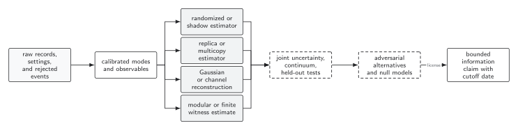
Entropy, tomography, witness, and recovery methods enter at the estimator stage, but all share calibration, uncertainty, continuum, and alternative-model tests. The final statement is no stronger than the least validated arrow. The diagram is schematic and not to scale.

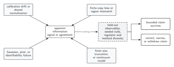
Different estimators can share the same calibration or normalization bias, so numerical agreement is not automatically independent replication. Adversarial nulls, held-out observables, regulator variation, and genuinely independent implementations set the claim ceiling and trigger correction when needed. The diagram is schematic.

References

• Monras, Alex, and Fabrizio Illuminati. “Measurement of Damping and Temperature: Precision Bounds in Gaussian Dissipative Channels.” Physical Review A 83 (2011): 012315. DOI. Open PDF.