Continuum Extrapolation, Bias, and Uncertainty

A QFT information uncertainty must combine finite samples, calibration, autocorrelation, discretization, finite volume, Hilbert or mode truncation, model discrepancy, and continuum extrapolation without treating correlated components as independent. The result is a distribution or bound for the final nonlinear quantity, together with an identification range for assumptions that data cannot resolve.

Required background. From Field Data to Information Claims supplies the inference chain.

Helpful background. Continuum Extrapolation and Finite-Time Windows supplies the joint cutoff, size, and time-window limit.

Decompose by source, combine through the pipeline

Write the reported estimator schematically as

$$\widehat I =F(D,C,\Lambda,V,N,M),$$

where $D$ are observations, $C$ calibration, $\Lambda$ lattice spacing or cutoff, $V$ volume, $N$ local/mode truncation, and $M$ the analysis and continuum model. Rather than adding separate error bars after evaluating $F$, resample or propagate these inputs jointly and recompute the entire estimator.

Classify uncertainties as:

• statistical: finite independent information after autocorrelation and batching;
• calibration: detector gains, control maps, switching, and region alignment;
• numerical: solver tolerance, Monte Carlo bias, truncation, and floating precision;
• regulator: cutoff, spacing, local Hilbert, and discretization family;
• finite extent: volume, time window, boundary, and recurrence effects;
• model: Gaussianity, fit ansatz, priors, neglected operators, or perturbative order;
• identification: range of target values among observationally compatible alternatives.

The last category is not reduced by more samples of the same observables.

Correlated resampling and continuum fitting

Suppose entropy estimates $S_{a,V,N}$ share raw configurations, calibration, or reference data. Estimate their joint covariance with block bootstrap, jackknife, or a generative likelihood that respects those dependencies. Fit a physically motivated form such as

$$S_{a,V,N} =S_\star+c_1a^p+c_2f_V(V)+c_3f_N(N)+c_{12}a^pf_V(V)+\cdots.$$

Do not add terms merely because they improve one fit. Specify the allowed correction orders before unblinding the final result where possible. Vary fit windows, correction families, covariance regularization, and regulator type. Model spread is reported separately or combined by a declared averaging rule.

The covariance matrix itself is uncertain and can be ill conditioned. Show eigenvalues, shrinkage or regularization, and stability. A diagonal fit to correlated points usually understates uncertainty.

Synthetic entropy propagation

For every resample:

1. draw experimental or simulation batches;
2. draw correlated calibration parameters;
3. reconstruct a physical covariance or evaluate the direct estimator;
4. apply nonlinear entropy transformations;
5. refit spacing, volume, and truncation dependence;
6. store the continuum target and diagnostics.

Inject a hidden calibration drift and test interval coverage across repeated synthetic datasets. Change the coarsest cutoff and correction exponent. If nominal 95% intervals cover far less often, expand the model or downgrade the claim.

Deterministic and probabilistic components

A rigorous truncation remainder can be combined with a statistical interval by enlarging the interval, while a subjective model ensemble should not be labeled a frequentist confidence level unless coverage is demonstrated. State the semantics of each component. The international metrology guide emphasizes a measurement model and covariance-aware propagation rather than an unqualified root-sum-square rule JCGM 2008, §§4–5.

As of 10 August 2026, continuum information estimates remain credible only where correlated calibration, regulator, volume, truncation, and model uncertainties have been propagated through the final nonlinear estimator and checked for coverage or stated as deterministic bounds.

Exercises

Shared calibration. Two estimators use the same uncertain detector gain. Can their gain errors be added independently?

Solution

No. Draw the common gain once per resample or include its covariance analytically. Independent draws would destroy the correlation and can either overstate or understate the uncertainty of their difference.

Fit-window drift. What does a systematic shift under removal of the coarsest regulator imply?

Solution

The asymptotic correction model or fit window is not yet stable. The shift belongs in model uncertainty, or the coarse points should be excluded by a criterion fixed and validated on benchmarks.

Inference and failure-control maps

The first diagram traces the complete path from raw records to a bounded information claim; inspect the assumption attached to every arrow. The second maps shared and method-specific failure channels to held-out tests, regulator variation, replication, and correction.

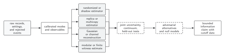
Entropy, tomography, witness, and recovery methods enter at the estimator stage, but all share calibration, uncertainty, continuum, and alternative-model tests. The final statement is no stronger than the least validated arrow. The diagram is schematic and not to scale.

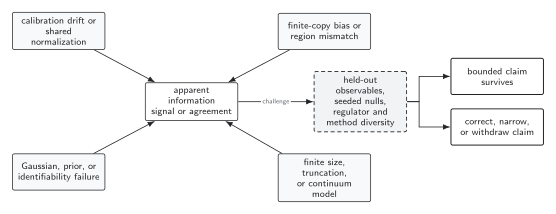
Different estimators can share the same calibration or normalization bias, so numerical agreement is not automatically independent replication. Adversarial nulls, held-out observables, regulator variation, and genuinely independent implementations set the claim ceiling and trigger correction when needed. The diagram is schematic.

References

• Joint Committee for Guides in Metrology. Evaluation of Measurement Data—Guide to the Expression of Uncertainty in Measurement. JCGM 100:2008. Official PDF.