Ball Regions and Conformal Modular Hamiltonians

For the vacuum of a conformal field theory, the modular flow of a round spatial ball is geometric and its modular Hamiltonian is a local stress-tensor charge. The result follows by conformally transporting the vacuum wedge flow to the ball’s causal diamond. The round geometry, conformal dynamics, and vacuum state are all essential.

Required background. Conformal geometry and maps supplies the wedge–diamond transformation, the conformal stress tensor supplies the conserved charge, and the Bisognano–Wichmann theorem fixes the wedge flow and its $2\pi$ normalization.

Helpful background. The cylinder map supplies the thermal-frame analogy, while CFT interval, sphere, and cylinder examples show how the same weight appears in entropy calculations.

The chapter’s route from standard pairs to geometric flow shows which step uses conformal covariance. Compare the ball row in the representative-flow table, and apply the claim-licensing checklist before changing the state, shape, or theory.

The conformal Killing field of the diamond

Let

$$B=\{\mathbf x:r<R\}, \qquad r=\lvert\mathbf x\rvert,$$

on the $t=0$ slice. Its domain of dependence is the diamond

$$D(B)=\{(t,\mathbf x):\lvert t\rvert+r<R\}.$$

With the site’s $(+---)$ metric, the future-directed conformal Killing field preserving this diamond is

$$\zeta_B= \frac{\pi}{R} \left[(R^2-t^2-r^2)\,\partial_t -2t x^i\partial_i\right].$$

Its squared norm is

$$\zeta_B^2= \frac{\pi^2}{R^2} \bigl[R^2-(t+r)^2\bigr] \bigl[R^2-(t-r)^2\bigr].$$

It is timelike inside the diamond and null on its boundary. It does not vanish at a generic boundary point. On the future boundary $t=R-r$,

$$\zeta_B= \frac{2\pi tr}{R}(\partial_t-\partial_r),$$

which is tangent to that null surface. The vector vanishes on the bifurcation sphere $(t=0,r=R)$ and at the two tips $(t=\pm R,r=0)$.

At $t=0$,

$$\zeta_B^0=\frac{\pi}{R}(R^2-r^2),$$

so the one-sided vacuum modular Hamiltonian is

$$\boxed{ K_B=2\pi\int_{r<R}d^{d-1}x\; \frac{R^2-r^2}{2R}\,T_{00}(0,\mathbf x)+c }.$$

The constant $c$ fixes $\operatorname{Tr}e^{-K_B}=1$ only in a regulated type-I representative. It does not affect the adjoint flow, and no such trace is required for the continuum ball algebra.

The shared wedge–ball diagram makes the conformal transport visible: inspect how wedge boost orbits bend into diamond-preserving ball trajectories while both entangling boundaries remain fixed.

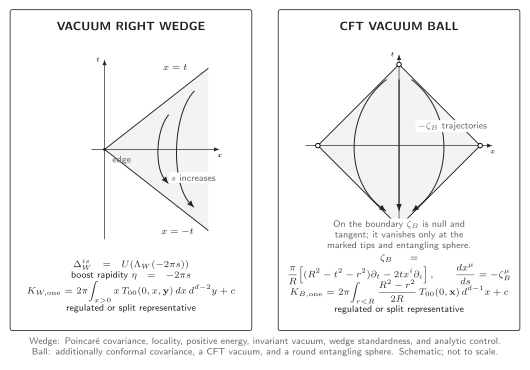
For the wedge, the geometric identification uses Poincaré covariance, locality, positive energy, an invariant vacuum, wedge standardness, and the analytic field control of the Bisognano–Wichmann theorem. For the ball it additionally uses conformal covariance, a CFT vacuum, and a round entangling sphere. The displayed stress-tensor charges are one-sided regulated or split representatives; the intrinsic continuum objects are the modular operators. With $\sigma_s=\operatorname{Ad}\Delta^{is}$, positive $s$ follows $\eta=-2\pi s$ in the wedge and $dx_s/ds=-\zeta_B$ in the ball. Schematic; not to scale.

The chapter sign convention

Use

$$\sigma_s(A)=\Delta_B^{is}A\Delta_B^{-is} =e^{-isK_B}Ae^{isK_B}.$$

The wedge page fixes positive modular time to rapidity $-2\pi s$. Conformal transport preserves this orientation. Therefore the spacetime point appearing in the transformed local operator obeys

$$\boxed{\frac{dx_s^\mu}{ds}=-\zeta_B^\mu(x_s)}.$$

The future-directed field $+\zeta_B$ instead generates the reversed convention $\widetilde\sigma_s=\Delta_B^{-is}(\,\cdot\,)\Delta_B^{is}$. This distinction does not change the positive weight in $K_B$: it records whether the adjoint action is written with $e^{-isK_B}$ or $e^{isK_B}$.

For a scalar primary $\mathcal O$ of dimension $\Delta_{\mathcal O}$,

$$\sigma_s(\mathcal O(x)) =\Omega_s(x)^{\Delta_{\mathcal O}}\mathcal O(x_s),$$

with the corresponding local Lorentz action on spin indices. The scale factor is fixed by the conformal map; it is not an arbitrary multiplier.

Deriving the flow from the wedge map

Write the diamond null coordinates as

$$x^+=r+t, \qquad x^-=r-t.$$

Transporting the Rindler boost through the special conformal map gives, in the site’s modular-time convention,

$$x_s^\pm= R\, \frac{(R+x^\pm)-e^{\pm2\pi s}(R-x^\pm)} {(R+x^\pm)+e^{\pm2\pi s}(R-x^\pm)}.$$

This is the $s\mapsto-s$ translation of the convention in Casini, Huerta, and Myers 2011, Eqs. (2.11)–(2.18), printed pp. 7–9. Differentiating at $s=0$ gives

$$\begin{aligned} \frac{dx^+_s}{ds}\bigg|_{0} &=-\frac{\pi}{R}\bigl[R^2-(x^+)^2\bigr],\\ \frac{dx^-_s}{ds}\bigg|_{0} &=+\frac{\pi}{R}\bigl[R^2-(x^-)^2\bigr]. \end{aligned}$$

Since $t=(x^+-x^-)/2$ and $r=(x^++x^-)/2$, these equations reproduce $dx_s/ds=-\zeta_B$ exactly.

A second derivation makes the kernel especially transparent. Introduce hyperbolic coordinates

$$\begin{aligned} t&=R\, \frac{\sinh(\tau/R)}{\cosh u+\cosh(\tau/R)},\\ r&=R\, \frac{\sinh u}{\cosh u+\cosh(\tau/R)},\\ \Omega&=\frac{1}{\cosh u+\cosh(\tau/R)}. \end{aligned}$$

Then

$$ds^2=\Omega^2 \left[d\tau^2-R^2\left(du^2+\sinh^2u\,d\Omega_{d-2}^2\right)\right].$$

The diamond restriction of the vacuum is mapped to a KMS state for $\tau$ translations with $T_{\mathrm{hyp}}=1/(2\pi R)$; “Gibbs density matrix” is regulated shorthand in continuum QFT Casini, Huerta, and Myers 2011, Eqs. (2.25)–(2.31), printed pp. 11–12. The site modular flow is

$$\tau\longmapsto\tau-2\pi Rs.$$

At $\tau=0$,

$$\frac rR=\tanh\frac u2, \qquad \frac{dt}{d\tau}=\frac{1}{1+\cosh u} =\frac{R^2-r^2}{2R^2}.$$

Consequently,

$$\frac{dt}{ds}\bigg|_{t=0} =-2\pi R\frac{dt}{d\tau} =-2\pi\frac{R^2-r^2}{2R},$$

which derives the stress-tensor weight and its $2\pi$ normalization rather than guessing it from symmetry.

Reproducible kernel check

Define $q=r/R$ and the dimensionless kernel

$$w(q)=\frac{1-q^2}{2}, \qquad K_B=2\pi\int_B d^{d-1}x\;R w(r/R)T_{00}+c.$$

$q$	$w(q)$	conclusion
$0$	$0.500$	maximum at the center
$0.5$	$0.375$	positive in the interior
$0.9$	$0.095$	approaching the Rindler regime
$1$	$0$	vanishes at the entangling surface

If $\delta=1-q$ is the inward proper distance in units of $R$, then

$$w(1-\delta)=\delta-\frac{\delta^2}{2}.$$

Thus the surface zero is linear and agrees with the half-space kernel to leading order. A reproducible implementation should report $q$, arithmetic precision, and

$$R_w(q)=\left\lvert w(q)-\frac{1-q^2}{2}\right\rvert.$$

The analytic target is $R_w=0$; a sampled table carries rounding uncertainty only. Checking positivity, the center value, the exact endpoint zero, and the linear coefficient catches sign, radius, and factor-of-two errors independently.

Adversarial relevant deformation

The conformal-map step fails sharply for a massive theory. For any conserved symmetric stress tensor and conformal Killing field,

$$\partial_\mu(T^{\mu\nu}\zeta_{B\nu}) =\frac{\partial\!\cdot\!\zeta_B}{d}\,T^\mu{}_{\mu}.$$

Here

$$\partial\!\cdot\!\zeta_B=-\frac{2\pi d}{R}t.$$

For a classically improved massive scalar in four dimensions, the on-shell trace is $T^\mu{}_{\mu}=m^2\phi^2$. Hence the would-be conformal current leaks by

$$\partial_\mu(T^{\mu\nu}\zeta_{B\nu}) =-\frac{2\pi t}{R}m^2\phi^2.$$

This is a direct failure of the conservation step used to identify $K_B$ with a conformal charge. As a normalized local test, choose a turning point of a homogeneous classical mode, where $\dot\phi=0$ and $T_{00}=m^2\phi^2/2$. At $t=R/4$,

$$L=\frac{\lvert\partial_\mu(T^{\mu\nu}\zeta_{B\nu})\rvert}{T_{00}} =\pi.$$

The nonzero leakage is exact for this classical control and does not depend on a numerical fit. At fixed field profile it scales as $m^2$. In a quantum calculation, $T^\mu{}_{\mu}$ and $\phi^2$ require a declared renormalization prescription; the relevant parameters include $mR$, the state, smearing scale, and scheme. This leakage test alone does not control an approximation to the modular Hamiltonian or its flow: a near-CFT or near-surface claim needs a separate observable-specific estimate with a stated topology and remainder.

Common pitfalls

Saying the vector vanishes on the null boundary. It becomes null and tangent there. Its actual zeros are the bifurcation sphere and the tips.

Following $+\zeta_B$ with the site’s $\Delta^{is}$ convention. The chapter convention follows $-\zeta_B$. Always display both the adjoint action and the trajectory equation.

Calling the hyperbolic KMS state a literal continuum density matrix. The intrinsic object is a state on the ball algebra. A trace and normalization constant belong to a regulator or split representative.

Exercises

1. Norm, tangency, and zeros

Starting from $\zeta_B$, derive its squared norm. Restrict the vector to $t=R-r$ and determine every zero on the closed diamond boundary.

Solution

The radial component is $\zeta^r=-2\pi tr/R$. Therefore

$$\begin{aligned} \zeta_B^2 &=\frac{\pi^2}{R^2} \left[(R^2-t^2-r^2)^2-4t^2r^2\right]\\ &=\frac{\pi^2}{R^2} \bigl[R^2-(t+r)^2\bigr] \bigl[R^2-(t-r)^2\bigr]. \end{aligned}$$

On $t=R-r$, $R^2-t^2-r^2=2tr$, so $\zeta_B=(2\pi tr/R)(\partial_t-\partial_r)$. This is tangent to the surface because $(\partial_t-\partial_r)(t+r-R)=0$. It vanishes when $tr=0$: the future tip $(R,0)$ or the bifurcation sphere $(0,R)$. The past boundary gives the past tip $(-R,0)$ and the same sphere.

2. Kernel from hyperbolic time

At $\tau=0$, prove $r/R=\tanh(u/2)$ and $dt/d\tau=(R^2-r^2)/(2R^2)$. Use $\tau\mapsto\tau-2\pi Rs$ to recover both the sign of the trajectory and the ball kernel.

Solution

At $\tau=0$,

$$\frac rR=\frac{\sinh u}{1+\cosh u}=\tanh\frac u2.$$

Differentiating $t$ gives $dt/d\tau=1/(1+\cosh u)$. If $q=\tanh(u/2)$, then $1/(1+\cosh u)=(1-q^2)/2=(R^2-r^2)/(2R^2)$. Therefore

$$\frac{dt}{ds}=-2\pi R\frac{dt}{d\tau} =-2\pi\frac{R^2-r^2}{2R}.$$

The minus sign agrees with $\sigma_s=e^{-isK_B}(\,\cdot\,)e^{isK_B}$, while the magnitude identifies the positive charge

$$K_B=2\pi\int_B\frac{R^2-r^2}{2R}T_{00}+c.$$

3. Trace-induced failure of conservation

Derive $\partial\!\cdot\!\zeta_B=-2\pi dt/R$. For an improved massive scalar with $T^\mu{}_{\mu}=m^2\phi^2$, compute the normalized leakage at $t=R/4$ and a turning point with $T_{00}=m^2\phi^2/2$. Which exact CFT step fails?

Solution

The time derivative contributes $-2\pi t/R$ and the $d-1$ spatial derivatives contribute $-2\pi(d-1)t/R$, giving $-2\pi dt/R$. The conformal-current Ward identity then gives

$$\left\lvert\partial_\mu(T^{\mu\nu}\zeta_{B\nu})\right\rvert =\frac{\pi}{2}m^2\phi^2$$

at $t=R/4$. Dividing by $T_{00}=m^2\phi^2/2$ yields $L=\pi$. The current is not conserved, so its charge cannot be transported as the exact wedge modular generator. Near-surface or small-$mR$ approximations may remain useful, but the exact conformal unitary equivalence has failed.

References

• Casini, Horacio, Marina Huerta, and Robert C. Myers. “Towards a Derivation of Holographic Entanglement Entropy.” Journal of High Energy Physics 2011, no. 5 (2011): 036. DOI; arXiv PDF.