Quasiparticle Pictures of Entanglement Growth

The quasiparticle picture explains entanglement growth when a quench creates spatially local groups of entangled excitations whose members then propagate approximately ballistically. It is more than a light-cone sketch: a quantitative prediction needs the entropy carried by each species and momentum, the post-quench velocity, and a statement of why scattering, decay, confinement, or multiparticle correlations can be neglected over the observed window.

Required background. Entanglement growth after quenches supplies the direct entropy data that the quasiparticle formula must predict rather than merely fit.

The interval formula

Consider a homogeneous one-dimensional quench and an interval $A$ of length $\ell$. For a low-entangled initial state in the joint space–time scaling limit $t,\ell\to\infty$ at fixed $t/\ell$, a convention that integrates over the full momentum domain gives the leading extensive term

$$S_A(t)= \sum_\alpha\int\frac{dk}{2\pi}\, s_\alpha(k)\min\!\left(2|v_\alpha(k)|t,\ell\right) +o(\ell).$$

$\alpha$ labels stable quasiparticle species, $s_\alpha(k)$ is the stationary entropy weight produced by the quench, and

$$v_\alpha(k)=\frac{\partial\varepsilon_\alpha(k)}{\partial k}$$

is the post-quench group velocity. The omitted $o(\ell)$ term contains finite-region, preparation-scale, and model-specific corrections; the display is not an exact finite-time identity. If one integrates over only half of momentum space or labels pairs rather than individual modes, the measure and entropy weight change. The invariant checks are that the late leading value equals the stationary entropy density times $\ell$ and that the early slope equals the entropy-weighted flux across both endpoints:

$$s_{\rm stat}=\sum_\alpha\int\frac{dk}{2\pi}s_\alpha(k), \qquad \left.\frac{dS_A}{dt}\right|_{\rm early} =2\sum_\alpha\int\frac{dk}{2\pi}|v_\alpha(k)|s_\alpha(k).$$

Why does the minimum appear? A pair born at $x$ with velocities $\pm v$ contributes when exactly one member is inside $A$. For one unoriented $\{k,-k\}$ pair type at early time, split pairs are born in a strip of width $2|v_k|t$ around each endpoint, so the geometric birth set has total measure $4|v_k|t$. In the displayed full-momentum convention, the $k$ and $-k$ entries carry equal weights; the same count therefore appears as the factor $2|v_k|t$ multiplying each entry. Once the two endpoint strips overlap, their symmetric difference has total measure $2\ell$, and the per-entry factor plateaus at $\ell$. The figure separates this geometry from the momentum-label convention.

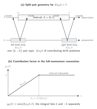
Quasiparticle counting for one interval in one spatial dimension. For one unoriented $\{k,-k\}$ pair type, each endpoint has a split-pair birth strip of width $2|v_k|t$; the full-momentum integral lists $k$ and $-k$ separately, giving $g_k(t)=\min(2|v_k|t,\ell)$ for each entry and a crossover at $t_k=\ell/(2|v_k|)$. The diagram is schematic and explains the leading scaling law, not an exact finite-time trajectory.

The pair-counting geometry was made explicit by Calabrese and Cardy 2005, § IV, Fig. 7 and Eq. (4.1), pp. 13–15. In an interacting integrable model, $s_\alpha$ is the Yang–Yang entropy contribution of the stationary macrostate and $v_\alpha$ is a dressed velocity, not the bare dispersion velocity. Alba and Calabrese 2017, Eqs. (2)–(3), pp. 7947–7949 formulate and test that generalized result in the space–time scaling limit.

Production entropy from a free mass quench

For the scalar quench defined on the contract page, the final-mode occupation is

$$n_k=\frac{(\omega_{f,k}-\omega_{i,k})^2} {4\omega_{f,k}\omega_{i,k}}.$$

The entropy of a bosonic mode with occupation $n$ is

$$h_{\rm B}(n)=(n+1)\log(n+1)-n\log n.$$

For a fermionic mode it is instead

$$h_{\rm F}(n)=-n\log n-(1-n)\log(1-n), \qquad 0\leq n\leq1.$$

These formulas are not interchangeable. Bosons have unbounded occupation and the $n\log n$ term is understood by continuity at $n=0$; fermions obey the exclusion bound. For an integrable Gaussian quench, the entropy weight $s(k)$ is fixed by the appropriate mode entropy, with any real-field pairing and momentum-domain convention handled consistently.

The lattice final dispersion and velocity are

$$\omega_{f,k}^2=m_f^2+\frac{4}{a^2}\sin^2\frac{ka}{2}, \qquad v_k=\frac{\sin(ka)}{a\omega_{f,k}}.$$

The largest group velocity is a property of this regulated dispersion. Replacing $v_k$ by one constant discards the slow modes that continue to contribute after the fastest front arrives and can distort both the initial slope and the rounded saturation crossover.

For the exact mode benchmark $(m_i,m_f,k)=(2,1,0)$, $n_0=1/8$ and

$$h_{\rm B}\!\left(\frac18\right) =\frac98\log\frac98-\frac18\log\frac18 \approx0.392436.$$

This is a mode entropy, not the entropy density. It must be integrated with the stated momentum measure. The distinction catches a common error in which a single-mode value is inserted as the coefficient of an extensive interval law.

Prediction against exact covariance data

The cleanest free-field test contains no entropy fit:

1. Use $(m_i,m_f,a,L)$ to calculate $n_k$, $h_{\rm B}(n_k)$, and $v_k$.
2. Insert these data into the quasiparticle integral with a frozen momentum convention.
3. Independently evolve the full covariance and calculate the symplectic spectrum of each interval.
4. Compare several $\ell$, both sides of the crossover, and more than one lattice spacing.
5. Propagate quadrature and finite-size errors rather than introducing an arbitrary overall normalization.

Cotler et al. 2016, §§ 3.1–3.3, pp. 15–24 perform this kind of comparison for free scalar fields in several dimensions and geometries. The leading large-region agreement is strong, while the zero-mode analysis in § 3.1, pp. 15–18 exhibits subleading information not contained in the simplest EPR-pair model.

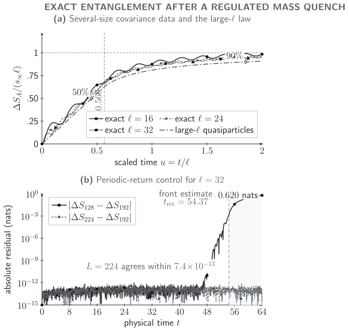
The finite-lattice comparison

The controlled several-size mass quench executes the five steps above with no fitted entropy normalization. It uses a periodic canonical chain with $(m_i,m_f,a,L)=(2,1,0.25,192)$, interval lengths $\ell=16,24,32$, analytic mode evolution sampled every $0.05$, and the independently calculated lattice density

$$s_\infty=0.1747729987.$$

Define the exact normalized curve and the parameter-free prediction by

$$F_\ell^{\rm exact}(u)=\frac{\Delta S_A(u\ell)}{s_\infty\ell}, \qquad F^{\rm QP}(u)=\frac{1}{s_\infty} \int_{-\pi/a}^{\pi/a}\frac{dk}{2\pi}\, h_B(n_k)\min(2|v_k|u,1).$$

At the predeclared ray $u=1$, the mode occupations and dispersion predict

$$F^{\rm QP}(1)=0.810127,$$

whereas exact covariance evolution gives

$$\bigl(F_{16}^{\rm exact}(1),F_{24}^{\rm exact}(1),F_{32}^{\rm exact}(1)\bigr) =(0.875131,0.867422,0.850375).$$

The corresponding absolute discrepancies are $0.065004$, $0.057295$, and $0.040248$. Their ordered decrease at this ray supports approach to the leading large-interval law, but three intervals at one spacing do not establish a convergence exponent or a continuum limit. A complementary threshold check makes the correction scale transparent: when each exact curve first crosses $0.9s_\infty\ell$, the exact-minus-leading difference remains about $0.23$–$0.24$ nats even though its fractional effect shrinks with $\ell$. That is the expected behavior of an order-one finite-interval correction to an order-$\ell$ prediction.

The volume, cutoff, sampling, purity, energy, symplectic, no-quench, and complement controls are recorded with the canonical calculation. The strongest statement that survives them is deliberately narrower than exact agreement: before periodic return, the exact curves exhibit a common early physical-time response and an approximately size-rescaled crossover toward the parameter-free quasiparticle law, with visible order-one coherent or boundary corrections. Download the canonical quantitative SVG, CSV curves and residuals, and JSON parameters, diagnostics, and claim boundary.

Continuum normalization as a separate check

The continuum integral is a useful normalization check, but it is not the same regulated problem. For $(m_i,m_f)=(2,1)$, $\omega_{r,k}=\sqrt{k^2+m_r^2}$, the full momentum line, and natural logarithms, composite Simpson quadrature on $0\leq k\leq1000$ gives

$$s_{\rm stat}\approx0.170612, \qquad 2\int\frac{dk}{2\pi}|v_k|s(k)\approx0.195864.$$

For $\ell=10$, the implied leading plateau is $10s_{\rm stat}\approx1.70612$, while the finite-time formula gives $S_A(10)\approx1.38389$. The gap is physical: slow modes with $2|v_k|t<\ell$ have not saturated. The continuum value $0.170612$ is about $2.4\%$ below the $a=0.25$ lattice value $0.174773$ because the dispersion and momentum domain differ at finite cutoff; it is not a contradictory normalization. The quoted Simpson calculation uses $2{,}000{,}000$ subintervals on the half-line. At fixed step size, extending the cutoff from $500$ to $1000$ changes the three displayed quantities by at most $1.2\times10^{-7}$; at fixed cutoff $1000$, doubling the subinterval count from $1{,}000{,}000$ changes them by at most $1.1\times10^{-8}$. Those are deterministic quadrature checks, not physical uncertainty estimates. This calculation checks the measure, bosonic entropy, velocity factor, and slow-mode tail, while the preceding finite-$a$ comparison tests the actual regulated covariance prediction.

A useful toy regression test replaces the integral by two already weighted sectors,

$$S(t)=\sum_{j=1}^2 s_j\min(2|v_j|t,\ell),$$

with $(s_1,s_2)=(0.1,0.2)$, $(v_1,v_2)=(1,0.5)$, and $\ell=4$. It gives $S(1)=0.4$ and $S(5)=1.2$. The first number checks the factor of two and velocity weighting; the second checks that the plateau is $\ell(s_1+s_2)$.

The more demanding test changes the post-quench dispersion while keeping the production profile as close as the model allows. The predicted front must move through $v_k$, whereas changing the initial mass at fixed final dispersion should primarily change the entropy weights. A formula that cannot distinguish those interventions is not using its microscopic inputs correctly.

Interacting integrable systems

In Bethe-ansatz-integrable models, stable quasiparticles scatter elastically but their propagation through a finite-density stationary state is dressed. Label a species and rapidity by $(\alpha,\lambda)$. The entropy formula becomes schematically

$$S_A(t)=\sum_\alpha\int d\lambda\, s_\alpha^{\rm YY}(\lambda) \min\!\left(2|v_\alpha^{\rm eff}(\lambda)|t,\ell\right),$$

where both the Yang–Yang entropy density and effective velocity are determined by the post-quench macrostate. Using the vacuum two-body group velocity in this finite-density problem generally fails. The success of the dressed formula links entanglement growth to generalized thermodynamics without asserting that the global pure state has acquired thermodynamic entropy.

The prediction still has a regime: homogeneous global quench, stable integrable quasiparticles, and the large-$t$, large-$\ell$ limit at fixed $t/\ell$, before finite-size return. Inhomogeneous states require local quasistationary data and generalized hydrodynamics. Boundary conditions, defects, and multiple production points modify the ray counting.

Broad multiparticle production: an exact stress test

The pair hypothesis can be changed without adding scattering or numerical uncertainty. Consider a dilute product of independent localized sources of density $\rho_3$. Each source emits three distinguishable two-level carriers in the GHZ state

$$|\mathrm{GHZ}_3\rangle =\frac{|000\rangle+|111\rangle}{\sqrt2}$$

with velocities $(-v,0,+v)$. Treat the wave packets as pointlike and ballistic over the observation window, neglect packet spreading and collisions, and let $A=[0,\ell]$. This is an exactly countable semiclassical source model, not a claim that the state is the ground state of a specified lattice Hamiltonian. Every nonempty proper subset of a GHZ triplet has entropy $\log2$, so a source contributes precisely when some, but not all, of its three carriers lie in $A$.

Write $d=vt$. A source born at $x$ has carriers at $x-d,x,x+d$. The birth positions for which at least one carrier lies in $A$ form

$$[-d,\ell-d]\cup[0,\ell]\cup[d,\ell+d],$$

while all three lie inside only for $x\in[d,\ell-d]$. Subtracting the intersection measure from the union measure gives the exact straddling length

$$g_3(t)= \begin{cases} 4vt, & 0\leq vt\leq\ell/2,\\ \ell+2vt, & \ell/2\leq vt\leq\ell,\\ 3\ell, & vt\geq\ell. \end{cases}$$

Thus $S_3(t)=\rho_3\log2\,g_3(t)$ and the late leading entropy density is $s_{\rm stat}=3\rho_3\log2$. Match that plateau with a frozen opposite-pair model by taking pair density $\rho_2=3\rho_3/2$, and use the same fastest carrier speed $v$. With $u=vt/\ell$, the pair prediction and exact triplet result are

$$F_{\rm pair}(u)=\min(2u,1), \qquad F_3(u)= \begin{cases} 4u/3, & 0\leq u\leq1/2,\\ (1+2u)/3, & 1/2\leq u\leq1,\\ 1, & u\geq1. \end{cases}$$

The predeclared comparison point is decisive:

$$F_{\rm pair}(1/2)=1, \qquad F_3(1/2)=\frac23.$$

The frozen pair law falsely declares saturation and overpredicts the exact answer by one third of the plateau, or $50\%$ relative to the triplet value. The mismatch is caused solely by the production-entanglement structure: the carriers remain stable and ballistic.

There is an important identifiability limit. Algebraically,

$$F_3(u)=\frac13\min(2u,1)+\frac23\min(u,1).$$

An unconstrained fit can therefore imitate this one-interval curve by inventing pair sectors with speeds $v$ and $v/2$. The test falsifies the microscopically frozen opposite-pair assignment, not every phenomenological sum of minimum functions. Independent information about the production amplitudes, carrier velocities, or multipartite correlations is what turns curve fitting into prediction.

This failure mechanism occurs in Hamiltonian quenches as well as in the analytic toy. Bastianello and Collura 2020, § 3, Eqs. (33) and (37)–(41), Figs. 2–3, pp. 8–13 study a tuned weak-interaction-to-free quench in which quartuplets survive while the leading pair amplitude is suppressed; the generalized multiplet prediction follows iTEBD data, whereas the occupation-matched pair ansatz misses the transient despite sharing the late plateau. Their perturbative construction concerns integer Rényi entropies and even multiplets. The GHZ calculation above is an independent von Neumann-entropy stress test, not a transcription of that model.

Strongest surviving claim. Ballistic ray counting survives; the frozen pair-production law does not. The interval entropy remains predictable only after the local multiplet state, not just its one-body occupations and maximum speed, is supplied.

Failure controls

Weakly break integrability. Add a tunable interaction that permits inelastic scattering. The integrable prediction may remain accurate for $t\ll\tau_{\rm scatt}$ and cross over later. Calling early agreement asymptotic hides the new scale.

Introduce confinement or instability. A quench across a confining perturbation can bind the presumed partners; an unstable excitation can decay into species with different velocities. Recalculate the spectrum and production channels rather than retaining the old pair picture.

Test more than the fastest edge. A maximum group velocity can predict the earliest support but not the entropy-weighted slope. Vary the interval and compare the full curve, including slow-mode tails.

Separate leading and subleading terms. Agreement of the volume-law contribution can coexist with universal or regulator-sensitive subleading structure. Fit the residual only after the leading prediction is frozen.

The chapter orientation map places this pair formula between microscopic input and direct entropy. Its failure controls identify dynamical-class transfer as a distinct error, and the diagnostic comparison states the window required for a quasiparticle claim.

Common pitfalls

Using the fastest velocity for every mode. The leading edge and the entropy slope weight the dispersion differently. Retain $v_\alpha(k)$ inside the integral.

Fitting the production entropy. In a predictive test, $s_\alpha$ comes from the initial state and stationary macrostate. An arbitrary scale factor removes the main physical content.

Calling all ballistic growth quasiparticle growth. Chaotic systems can also have a linear entropy regime. The evidence for quasiparticles is a successful mode-resolved prediction and its controlled failure when stability or integrability is broken.

Exercises

Assume a single species with speed $v$ and integrated entropy density $s$. Evaluate the pair formula before and after $t=\ell/(2v)$.

Solution

With only one speed, the integral reduces to

$$S_A(t)-S_A(0)=s\min(2vt,\ell).$$

It grows as $2svt$ for $t<\ell/(2v)$ and saturates at $s\ell$ afterward. The two branches meet continuously at the crossover.

For the bosonic occupation $n=1/8$, calculate $h_{\rm B}(n)$ and compare it with the fermionic entropy formula evaluated at the same numerical $n$.

Solution

The bosonic value is

$$h_{\rm B}=\frac98\log\frac98-\frac18\log\frac18 \approx0.392436.$$

The fermionic value is

$$h_{\rm F}=-\frac18\log\frac18-\frac78\log\frac78 \approx0.376770.$$

Their numerical closeness at small occupation does not make them equivalent; the Hilbert-space statistics and allowed range of $n$ differ.

Use the two-sector benchmark $(s_1,s_2)=(0.1,0.2)$, $(v_1,v_2)=(1,0.5)$, and $\ell=4$. Find the times at which each sector saturates and write $S(t)$ piecewise.

Solution

Sector 1 saturates at $t_1=\ell/(2v_1)=2$; sector 2 saturates at $t_2=4$. Thus

$$S(t)= \begin{cases} 0.4t, & 0\leq t\leq2,\\ 0.4+0.2t, & 2\leq t\leq4,\\ 1.2, & t\geq4. \end{cases}$$

At $t=1$, $S=0.4$; by $t=5$, both sectors have saturated and $S=1.2$.

At $u=1$, the lattice quasiparticle prediction is $F^{\rm QP}=0.810127$, while exact covariance evolution gives $F_\ell^{\rm exact}=0.875131$, $0.867422$, and $0.850375$ for $\ell=16$, $24$, and $32$. Calculate the three absolute discrepancies. What conclusion is licensed by their size dependence?

Solution

Subtracting the frozen prediction gives

$$\delta_{16}=0.065004, \qquad \delta_{24}=0.057295, \qquad \delta_{32}=0.040248.$$

The discrepancy decreases across these three intervals at the tested ray, which supports approach to the leading large-$\ell$ quasiparticle law. It does not determine a correction exponent, prove convergence at every $u$, or establish a continuum limit because only one lattice spacing and three interval sizes enter this comparison.

Show that the exact triplet curve can be written as

$$F_3(u)=\frac13\min(2u,1)+\frac23\min(u,1),$$

and explain why this identity limits what a one-interval entropy curve can reveal about the production state.

Solution

For $0\leq u\leq1/2$, both minimum functions are unsaturated, so the right-hand side is $2u/3+2u/3=4u/3$. For $1/2\leq u\leq1$, the first is saturated and the second is not, giving $(1+2u)/3$. For $u\geq1$, both are saturated and the result is $1$. These are exactly the three branches of $F_3$.

Consequently, an unconstrained pair fit can reproduce the triplet curve by assigning positive weights to apparent speed sectors $v$ and $v/2$. Interval entropy alone therefore rejects the triplet’s frozen microscopic opposite-pair prediction, but it cannot distinguish the triplet from every fitted pair mixture. Production amplitudes, known velocities, or a genuinely multipartite diagnostic are also needed.

References

• Alba, Vincenzo, and Pasquale Calabrese. “Entanglement and Thermodynamics after a Quantum Quench in Integrable Systems.” Proceedings of the National Academy of Sciences 114 (2017): 7947–7951. DOI.
• Bastianello, Alvise, and Mario Collura. “Entanglement Spreading and Quasiparticle Picture beyond the Pair Structure.” SciPost Physics 8 (2020): 045. DOI.
• Calabrese, Pasquale, and John Cardy. “Evolution of Entanglement Entropy in One-Dimensional Systems.” Journal of Statistical Mechanics: Theory and Experiment 2005 (2005): P04010. DOI.
• Cotler, Jordan S., Mark P. Hertzberg, Márk Mezei, and Mark T. Mueller. “Entanglement Growth after a Global Quench in Free Scalar Field Theory.” Journal of High Energy Physics 2016, no. 11 (2016): 166. DOI.