Strong Subadditivity and Entropic Inequalities

Strong subadditivity answers a precise question: when do four subregion entropies form one regulator-consistent inequality? They do when the regions are compatible restrictions of one state. At a finite type-I regulator the resulting conditional mutual information is exactly the distinguishability lost by discarding a subsystem; in continuum QFT, only a common-regulator limit or an algebraic relative-entropy formulation has that meaning.

Required background. Use regulated subregion entropy. Helpful background. Positivity, Monotonicity, and Data Processing supplies the relative-entropy proof strategy.

The chapter’s task-comparison table separates this entropy inequality from the additional channel and error estimates needed for a recovery theorem.

Strong subadditivity as lost distinguishability

Let $\rho_{ABC}$ be a normalized state on a finite-dimensional tensor product $\mathcal H_A\otimes\mathcal H_B\otimes\mathcal H_C$. For density operators $\rho$ and $\sigma$, the Umegaki relative entropy is

$$D(\rho\Vert\sigma)= \begin{cases} \operatorname{Tr}\rho(\log\rho-\log\sigma), & \operatorname{supp}\rho\subseteq\operatorname{supp}\sigma,\\ +\infty, & \text{otherwise}. \end{cases}$$

Apply data processing to the channel $\Phi=\operatorname{Tr}_C$ and, importantly, to the same two states before and after the channel:

$$\begin{aligned} \rho&=\rho_{ABC}, &\sigma&=\rho_A\otimes\rho_{BC},\\ \Phi(\rho)&=\rho_{AB}, &\Phi(\sigma)&=\rho_A\otimes\rho_B. \end{aligned}$$

Because $\operatorname{supp}\rho_{ABC}\subseteq\operatorname{supp}\rho_A\otimes\operatorname{supp}\rho_{BC}$ and $\operatorname{supp}\rho_{AB}\subseteq\operatorname{supp}\rho_A\otimes\operatorname{supp}\rho_B$, both relative entropies below are finite; no full-rank or faithfulness assumption is required. Data processing gives

$$D(\rho_{ABC}\Vert\rho_A\otimes\rho_{BC}) \geq D(\rho_{AB}\Vert\rho_A\otimes\rho_B).$$

Expanding the logarithms shows exactly what was lost:

$$\begin{aligned} D(\rho_{ABC}\Vert\rho_A\otimes\rho_{BC}) &=S(A)+S(BC)-S(ABC),\\ D(\rho_{AB}\Vert\rho_A\otimes\rho_B) &=S(A)+S(B)-S(AB). \end{aligned}$$

Consequently,

$$\boxed{ I(A{:}C\mid B) =D(\rho_{ABC}\Vert\rho_A\otimes\rho_{BC}) -D(\rho_{AB}\Vert\rho_A\otimes\rho_B) \geq0 }$$

with

$$I(A{:}C\mid B) =S(AB)+S(BC)-S(B)-S(ABC).$$

Thus the sign is “before minus after”: $I(A{:}C\mid B)=I(A{:}BC)-I(A{:}B)$. A product such as $\rho_{AB}\otimes\rho_{BC}$ is not a valid substitute for the reference state because it duplicates $B$ and acts on the wrong Hilbert space. This exact reduction appears in Hayden et al. 2004, § III, equations (4)–(7); finite-dimensional data processing was proved by Lindblad 1975, pp. 147–151, and strong subadditivity itself by Lieb and Ruskai 1973, Theorem 2, equations (1.5)–(1.6).

The structure diagram places this result between correlation measures and recovery: nonnegativity is automatic under the hypotheses above, while equality and approximation require further structure.

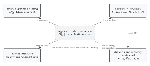
Strong subadditivity identifies conditional mutual information as a nonnegative correlation quantity for one compatible tripartite state. Exact or approximate recovery requires the additional equality, support, and channel statements developed later. Schematic.

Consequences and their hypotheses

The same inequality can be written as monotonicity of conditional entropy,

$$S(A\mid B)\geq S(A\mid BC), \qquad S(A\mid B)=S(AB)-S(B).$$

Taking the middle system to be trivial gives subadditivity for every finite-dimensional bipartite state,

$$S(AB)\leq S(A)+S(B).$$

Another consequence is weak monotonicity,

$$S(AB)+S(BC)\geq S(A)+S(C),$$

or $S(B\mid A)+S(B\mid C)\geq0$. To see it without memorizing a second theorem, purify $\rho_{ABC}$ to $\lvert\psi\rangle_{ABCD}$ and apply strong subadditivity to $B$–$A$–$D$:

$$S(AB)+S(AD)\geq S(A)+S(ABD).$$

Purity gives $S(AD)=S(BC)$ and $S(ABD)=S(C)$, which is the claimed inequality.

For any finite-dimensional bipartite state, the Araki–Lieb and subadditivity bounds combine into

$$\lvert S(A)-S(B)\rvert\leq S(AB)\leq S(A)+S(B).$$

For the lower bound, purify $AB$ by $C$ and apply subadditivity to $BC$:

$$S(A)=S(BC)\leq S(B)+S(C)=S(B)+S(AB).$$

This proves $S(A)-S(B)\leq S(AB)$; exchanging $A$ and $B$ supplies the other sign. No purity assumption is made about $\rho_{AB}$. The original result and its infinite-dimensional hypotheses are given by Araki and Lieb 1970, pp. 160–170.

None of these inequalities makes entropy monotone under inclusion. If $AB$ is a Bell pair, then $S(A)=\log2$ while $S(AB)=0$: adding $B$ purifies rather than increases the entropy. What is monotone here is relative entropy under a channel, not the entropy of an arbitrarily enlarged subsystem.

Overlapping regions and endpoint-local cancellation

At a common type-I regulator, overlapping regions $U$ and $V$ can be decomposed as $U=A\cup B$ and $V=B\cup C$, where $B=U\cap V$. Strong subadditivity then has the geometric form

$$S(U)+S(V)\geq S(U\cap V)+S(U\cup V).$$

This identification requires the displayed regions to correspond to compatible subsystem factors or algebra restrictions. A set-theoretic drawing alone does not establish the required quantum-algebra relations.

For three adjacent intervals, write the four physical cuts as

$$x_0\mid A\mid x_1\mid B\mid x_2\mid C\mid x_3.$$

If $u(x_i,a)$ denotes any endpoint-local ultraviolet term produced by one common cutoff $a$, its signed coefficient in the conditional mutual information is:

Physical cut	$+S(AB)$	$+S(BC)$	$-S(B)$	$-S(ABC)$	Net coefficient
$x_0$	$+1$	$0$	$0$	$-1$	$0$
$x_1$	$0$	$+1$	$-1$	$0$	$0$
$x_2$	$+1$	$0$	$-1$	$0$	$0$
$x_3$	$0$	$+1$	$0$	$-1$	$0$

Every local endpoint contribution cancels against the same contribution evaluated with the same prescription. As an analytic check, consider the vacuum of a 1+1-dimensional CFT on the infinite line. For a single interval,

$$S(\ell)=\frac{c}{3}\log\frac{\ell}{\epsilon}+s_0.$$

For adjacent lengths $x$, $y$, and $z$, with $y>0$,

$$\begin{aligned} I(A{:}C\mid B) &=\frac{c}{3}\log\frac{(x+y)(y+z)}{y(x+y+z)}\\ &=\frac{c}{3}\log\left(1+\frac{xz}{y(x+y+z)}\right)\geq0. \end{aligned}$$

The cutoff and additive constant cancel, and positivity follows because the numerator exceeds the denominator by $xz$. The expression diverges as the physical buffer $y$ shrinks to zero, so a cutoff refinement must hold $y$ fixed rather than hold its site count fixed. The interval formula is derived in Calabrese and Cardy 2004, § III.A, equation (16).

What survives the continuum limit

At every finite common regulator, the theorem applies directly. In continuum QFT, however, sharp local algebras are generally not type I, individual subregion entropies are ultraviolet divergent, and a four-term expression may otherwise be an undefined subtraction of infinities. One must either take the limit of the complete common-regulator combination and demonstrate convergence, or use relative entropy for compatible von Neumann-algebra restrictions. Araki 1975, pp. 809–833 proves monotonicity for algebraic relative entropy; Casini 2004, § II–III explains the geometric entropy inequalities and the localization caveat. A rigorous operator-algebra route begins with noncommutative divergences and information bounds.

Gauge constraints make the subsystem choice especially consequential: a spatial region need not determine a tensor factor, and center or edge-mode choices change the entropy decomposition. The same compatible algebra prescription must therefore be used in all four terms. Casini, Huerta, and Rosabal 2014, §§ 4 and 6 analyze these boundary-algebra ambiguities. In higher dimensions, cancellation of a leading area term alone is not enough; corner, junction, curvature, center, and edge contributions must also pair before a finite limit is claimed.

The following diagram distinguishes a valid common-system comparison from combinations assembled using incompatible states, regulators, or boundary prescriptions.

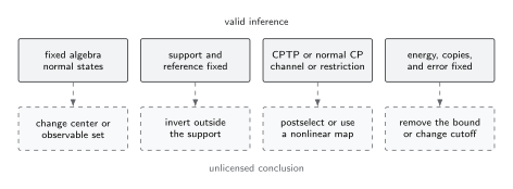
All four entropy terms must be restrictions of one state under one compatible subsystem prescription. Mixing lattice spacings, endpoint assignments, edge-mode conventions, or centers can leave unmatched boundary terms and does not test strong subadditivity. Schematic.

Periodic massive-chain benchmark

A quantitative check uses the ground state of the periodic harmonic chain

$$H_N=\frac12\sum_{n=0}^{N-1} \left[ p_n^2+m^2q_n^2+\frac{(q_{n+1}-q_n)^2}{a^2} \right],$$

with $[q_n,p_r]=i\delta_{nr}$, $q_N=q_0$, circumference $L=Na=32$, and mass $m=1$. Sites are cell-centered and interval boundaries lie on cell edges. The physical lengths are held fixed at

$$(\ell_A,\ell_B,\ell_C)=(2,1,2),$$

so each refinement uses exactly $(n_A,n_B,n_C)=(2/a,1/a,2/a)$ consecutive, nonwrapping sites. This is a refinement of one geometry, not a sequence with shrinking physical intervals.

The normal-mode frequencies and ground-state covariance matrices are

$$\begin{aligned} \omega_k&=\sqrt{m^2+\frac{4}{a^2}\sin^2\frac{\pi k}{N}},\\ X_{ij}&=\frac{1}{2N}\sum_{k=0}^{N-1} \frac{\cos[2\pi k(i-j)/N]}{\omega_k},\\ P_{ij}&=\frac{1}{2N}\sum_{k=0}^{N-1} \omega_k\cos[2\pi k(i-j)/N]. \end{aligned}$$

For a region $R$, restrict $X$ and $P$ to $X_R$ and $P_R$. Numerically diagonalize the symmetric positive matrix

$$M_R=X_R^{1/2}P_RX_R^{1/2}, \qquad \nu_j=\sqrt{\lambda_j(M_R)}\geq\frac12,$$

rather than a nonsymmetric floating-point representation of $X_RP_R$. With natural logarithms, the entropy in nats is

$$S(R)=\sum_j \left[ \left(\nu_j+\frac12\right)\log\left(\nu_j+\frac12\right) -\left(\nu_j-\frac12\right)\log\left(\nu_j-\frac12\right) \right],$$

where $0\log0$ is evaluated by continuity. These covariance and entropy formulas follow Casini and Huerta 2009, equations (63), (65), (66), and (197)–(199).

The reproducible benchmark record contains the parameters, conventions, component entropies, and conditional mutual information. The refinement gives:

$N$	$a$	$(n_A,n_B,n_C)$	$S(AB)=S(BC)$	$S(B)$	$S(ABC)$	$I(A{:}C\mid B)$
$256$	$0.125$	$(16,8,16)$	$0.696883239$	$0.682098058$	$0.697037991$	$0.014630429$
$512$	$0.0625$	$(32,16,32)$	$0.925183388$	$0.910429334$	$0.925337478$	$0.014599965$
$1024$	$0.03125$	$(64,32,64)$	$1.155417401$	$1.140672423$	$1.155571327$	$0.014591052$

The individual entropies grow under refinement, while their common-regulator combination converges. Successive $a^2$ Richardson estimates from the $(256,512)$ and $(512,1024)$ pairs are $0.0145898103$ and $0.0145880808$. Taking $1.2$ times their difference as a deliberately conservative cutoff-sensitivity envelope gives

$$I(A{:}C\mid B)_{a\to0}=0.0145881\pm0.0000021 \quad\text{nats}.$$

The uncertainty is an observed discretization envelope, not a statistical error bar or a rigorous error bound. The record checks covariance symmetry, the global purity identity $XP=I/4$, $\nu_j\geq1/2$ up to documented roundoff-scale deficits, translation invariance, $S(AB)=S(BC)$, and a fixed-$a$ finite-volume spread below $5.0\times10^{-12}$ nats. An independent NumPy diagonalization reproduced the displayed rows within $2\times10^{-9}$ nats.

An adversarial mismatch

Now take the positive terms from $N=256$ but the negative terms from $N=512$:

$$\begin{aligned} I_{\mathrm{mixed}} &=S_{256}(AB)+S_{256}(BC)-S_{512}(B)-S_{512}(ABC)\\ &=2(0.696883238792)-0.910429333573-0.925337478087\\ &=-0.442000334076. \end{aligned}$$

This negative number is not a conditional mutual information. Its four terms are not marginals of one state on one tensor decomposition, so no channel maps the required before-pair to the after-pair and data processing does not apply. It diagnoses a mismatched calculation, not a failure of strong subadditivity.

Equality and the Markov handoff

In finite dimension, $I(A{:}C\mid B)=0$ if and only if $B$ decomposes as

$$\mathcal H_B=\bigoplus_j \mathcal H_{B_L^j}\otimes\mathcal H_{B_R^j}$$

and

$$\rho_{ABC}=\bigoplus_j p_j\, \rho_{A B_L^j}\otimes\rho_{B_R^j C}.$$

Equivalently, a recovery channel from $B$ to $BC$ reconstructs $\rho_{ABC}$ from $\rho_{AB}$. This statement requires no faithful state; the explicit Petz map uses inverses only on the relevant supports and can be extended off them. Petz 1986, pp. 123–131 gives the sufficiency criterion, and Hayden et al. 2004, § V, Theorem 6 gives the finite-dimensional direct-sum form. Conditional Mutual Information and Quantum Markov Structure develops the equality case and explains why small, rather than zero, conditional mutual information calls for an approximate recovery theorem.

Common pitfalls

Reversing the data-processing loss. Strong subadditivity is “relative entropy before tracing out $C$ minus relative entropy afterward.” Reversing that order manufactures the wrong sign.

Treating entropy as monotone under inclusion. A larger subsystem can have smaller entropy, as the Bell-pair example shows. The monotone object in the proof is relative entropy under a channel.

Mixing four individually plausible numbers. Each entropy may be accurately computed and the combination can still be meaningless if the state, cutoff, endpoints, or center prescription differs between terms. Verify the common parent state before interpreting the sign.

Exercises

1. Recover the sign and reference pair

Starting from data processing under $\operatorname{Tr}_C$, derive strong subadditivity and explain why $\rho_{AB}\otimes\rho_{BC}$ cannot be the reference state.

Solution

Choose $\rho=\rho_{ABC}$ and $\sigma=\rho_A\otimes\rho_{BC}$. Partial trace sends them to $\rho_{AB}$ and $\rho_A\otimes\rho_B$, respectively. Therefore

$$D(\rho_{ABC}\Vert\rho_A\otimes\rho_{BC}) -D(\rho_{AB}\Vert\rho_A\otimes\rho_B)\geq0.$$

Expanding gives $S(AB)+S(BC)-S(B)-S(ABC)\geq0$. The alternative $\rho_{AB}\otimes\rho_{BC}$ contains two copies of $B$, acts on $ABBC$, and is not a state on the original $ABC$ system.

2. Derive two purification consequences

Use purification and subadditivity or strong subadditivity to prove weak monotonicity and the Araki–Lieb lower bound.

Solution

Purify $ABC$ by $D$. Strong subadditivity on $B$–$A$–$D$ gives

$$S(AB)+S(AD)\geq S(A)+S(ABD).$$

Using $S(AD)=S(BC)$ and $S(ABD)=S(C)$ yields weak monotonicity. Separately, purify $AB$ by $C$ and apply subadditivity to $BC$:

$$S(A)=S(BC)\leq S(B)+S(C)=S(B)+S(AB).$$

Thus $S(A)-S(B)\leq S(AB)$; exchange $A$ and $B$ and combine the two inequalities to obtain $\lvert S(A)-S(B)\rvert\leq S(AB)$.

3. Check the CFT cancellation

For adjacent interval lengths $x,y,z>0$, insert $S(\ell)=\frac c3\log(\ell/\epsilon)+s_0$ into the four-term conditional mutual information. Prove positivity and determine the $y\to0^+$ behavior.

Solution

The two cutoff terms and two constants cancel, leaving

$$I(A{:}C\mid B) =\frac c3\log\frac{(x+y)(y+z)}{y(x+y+z)}.$$

Since $(x+y)(y+z)-y(x+y+z)=xz>0$, the logarithm is positive. For small $y$, its argument behaves as $xz/[y(x+z)]$, so the conditional mutual information diverges logarithmically.

4. Diagnose the negative mixed-cutoff number

Use the $N=256$ values for $S(AB)$ and $S(BC)$ and the $N=512$ values for $S(B)$ and $S(ABC)$. Why does the result not contradict the theorem?

Solution

The substitution gives

$$2(0.696883238792)-0.910429333573-0.925337478087 =-0.442000334076.$$

Strong subadditivity compares four marginals of one density operator. Here the terms come from different lattice Hilbert spaces and different global ground states, so they do not define any single $I(A{:}C\mid B)$. The negative value exposes the incompatible regulator assignment.

References

• Araki, Huzihiro. “Relative Entropy of States of von Neumann Algebras.” Publications of the Research Institute for Mathematical Sciences 11, no. 3 (1975): 809–833. DOI.
• Araki, Huzihiro, and Elliott H. Lieb. “Entropy Inequalities.” Communications in Mathematical Physics 18, no. 2 (1970): 160–170. DOI.
• Calabrese, Pasquale, and John Cardy. “Entanglement Entropy and Quantum Field Theory.” Journal of Statistical Mechanics: Theory and Experiment 2004, no. 6 (2004): P06002. DOI. Open PDF.
• Casini, Horacio. “Geometric Entropy, Area, and Strong Subadditivity.” Classical and Quantum Gravity 21, no. 9 (2004): 2351–2378. DOI. Open PDF.
• Casini, Horacio, and Marina Huerta. “Entanglement Entropy in Free Quantum Field Theory.” Journal of Physics A: Mathematical and Theoretical 42, no. 50 (2009): 504007. DOI. Open PDF.
• Casini, Horacio, Marina Huerta, and José Alejandro Rosabal. “Remarks on Entanglement Entropy for Gauge Fields.” Physical Review D 89, no. 8 (2014): 085012. DOI. Open PDF.
• Hayden, Patrick, Richard Jozsa, Dénes Petz, and Andreas Winter. “Structure of States Which Satisfy Strong Subadditivity of Quantum Entropy with Equality.” Communications in Mathematical Physics 246, no. 2 (2004): 359–374. DOI. Open PDF.
• Lieb, Elliott H., and Mary Beth Ruskai. “Proof of the Strong Subadditivity of Quantum-Mechanical Entropy.” Journal of Mathematical Physics 14, no. 12 (1973): 1938–1941. DOI. Expanded open version.
• Lindblad, Göran. “Completely Positive Maps and Entropy Inequalities.” Communications in Mathematical Physics 40, no. 2 (1975): 147–151. DOI.
• Petz, Dénes. “Sufficient Subalgebras and the Relative Entropy of States of a von Neumann Algebra.” Communications in Mathematical Physics 105, no. 1 (1986): 123–131. DOI. Open PDF.