Relative Entropy for QFT States

Relative entropy asks how well two states can be distinguished using the observables in one declared algebra. This algebra-first definition is the natural one in continuum QFT: it works for type-III local algebras, needs no reduced density matrix or local trace, and often remains finite even when the individual local von Neumann entropies do not exist. The order matters throughout: $S(\omega\Vert\varphi)$ treats $\omega$ as the state being tested and $\varphi$ as the reference.

Required background. Use operator algebras and normal positive functionals and restricted states on subregions. Helpful background. Type-III local algebras explain why the density-matrix formula is not the continuum definition.

Before applying a formula, use the chapter’s validity map to check algebra, support, regulator, and resource assumptions. The claim-comparison table separates algebraic relative entropy from hypothesis testing, fidelity, recovery, and channel distances.

The algebraic comparison

Let $\omega$ and $\varphi$ be normal states on a von Neumann algebra $\mathfrak M$. In standard form, let $\xi_\omega$ and $\xi_\varphi$ be their natural-cone representatives. For faithful states, close the antilinear operator

$$\mathsf S_{\varphi\mid\omega,0}(x\xi_\omega)=x^*\xi_\varphi, \qquad x\in\mathfrak M,$$

and define

$$\Delta_{\varphi,\omega} =\mathsf S_{\varphi\mid\omega}^*\mathsf S_{\varphi\mid\omega}.$$

With the second state as reference,

$$S_{\mathfrak M}(\omega\Vert\varphi) =-\langle\xi_\omega, \log\Delta_{\varphi,\omega}\,\xi_\omega\rangle.$$

Araki’s extension to arbitrary normal states incorporates their support projections and interprets the logarithm spectrally. If $s(\omega)\nleq s(\varphi)$, the value is $+\infty$. If support inclusion holds, the logarithmic quadratic form may still diverge in infinite dimensions. See Araki 1976, Eqs. (1.1)–(1.2), p. 809 and Araki 1977, Definition 3.1 and Remarks 3.4–3.5, pp. 177–178.

For normalized normal states,

$$S_{\mathfrak M}(\omega\Vert\varphi)\geq0,$$

with equality exactly when $\omega=\varphi$ as states on the declared algebra; see Araki 1977, Theorem 3.6(1), pp. 178–179.

The density-matrix expression follows from this construction rather than replacing it. For faithful density matrices $\rho$ and $\sigma$ on a finite-dimensional Hilbert space, represent $\mathcal B(\mathcal H)$ on Hilbert–Schmidt operators and write $\xi_\rho=\rho^{1/2}$. Then

$$\Delta_{\sigma,\rho}=L_\sigma R_{\rho^{-1}},$$

where $L_a(X)=aX$ and $R_b(X)=Xb$. Left and right multiplication commute, so

$$\log\Delta_{\sigma,\rho} =L_{\log\sigma}-R_{\log\rho}.$$

Consequently,

$$\begin{aligned} -\langle\rho^{1/2}, \log\Delta_{\sigma,\rho}\,\rho^{1/2}\rangle_{\mathrm{HS}} &=-\operatorname{Tr}\rho\log\sigma +\operatorname{Tr}\rho\log\rho\\ &=\operatorname{Tr}\rho(\log\rho-\log\sigma). \end{aligned}$$

After extending to nonfaithful finite-dimensional matrices,

$$D(\rho\Vert\sigma)= \begin{cases} \operatorname{Tr}\rho(\log\rho-\log\sigma), &\operatorname{supp}\rho\leq\operatorname{supp}\sigma,\\[2pt] +\infty,&\text{otherwise}. \end{cases}$$

For trace-class density operators on an infinite-dimensional Hilbert space, the first branch means the extended Umegaki functional, not a subtraction of two separately infinite traces. Support inclusion removes the automatic singular branch but does not guarantee a finite value.

For commuting matrices it is simply the classical Kullback–Leibler divergence $\sum_i p_i\log(p_i/q_i)$. For noncommuting QFT states, the relative modular operator is the replacement for the ratio $p_i/q_i$.

What distinguishability means locally

The algebra $\mathfrak M$ specifies which measurements are allowed. For a finite-outcome POVM $\{E_i\}\subset\mathfrak M$, define $p_i=\omega(E_i)$ and $q_i=\varphi(E_i)$. Data processing gives

$$D(p\Vert q)\leq S_{\mathfrak M}(\omega\Vert\varphi).$$

Thus algebraic relative entropy bounds the classical distinguishability available to every such local measurement; it is not itself a one-shot error probability and need not be attained by one measurement. A many-copy error exponent requires an explicitly declared product-state experiment, treated on Hypothesis Testing and Asymptotic Distinguishability.

Likewise, if $\mathfrak N\subset\mathfrak M$ is a genuine inclusion and both pairs are literal restrictions of the same two states, then

$$S_{\mathfrak N}(\omega|_{\mathfrak N}\Vert\varphi|_{\mathfrak N}) \leq S_{\mathfrak M}(\omega\Vert\varphi).$$

This statement does not compare unrelated cutoff systems; its proof and channel form belong to Positivity, Monotonicity, and Data Processing. Two globally different preparations can nevertheless have $S_{\mathfrak M}=0$ when their restrictions agree on $\mathfrak M$. Relative entropy compares states as seen by the stated observer, not vectors in an unspecified global Hilbert space.

The diagram shows which conclusions start from the same algebraic core and which extra inputs they need.

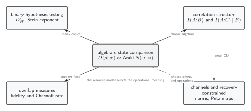
Araki relative entropy is the central state comparison. Hypothesis tests, overlap bounds, mutual information, and recovery statements are related but distinct tasks with their own copy, algebra, channel, and resource assumptions. Schematic.

The type-I modular balance

For faithful density matrices, define the reference modular Hamiltonian $K_\sigma=-\log\sigma$ and

$$\Delta\langle K_\sigma\rangle =\operatorname{Tr}(\rho-\sigma)K_\sigma, \qquad \Delta S=S_{\mathrm{vN}}(\rho)-S_{\mathrm{vN}}(\sigma).$$

When the displayed traces are defined and finite, a direct rearrangement gives

$$D(\rho\Vert\sigma) =\Delta\langle K_\sigma\rangle-\Delta S.$$

At each finite type-I regulator this identity is exact. It does not prove that a sequence of regulators converges: identifying a cutoff limit with continuum Araki relative entropy requires compatible algebras and states plus an applicable convergence theorem, as explained on Araki Relative Entropy and Regulated Limits. On a type-III algebra, the separate regulated quantities $\Delta\langle K\rangle$ and $\Delta S$ must not be promoted to intrinsic local von Neumann entropies.

At a finite Gaussian regulator, a Weyl displacement changes first moments but not covariance, so the displaced state and its reference have identical reduced Gaussian entropy and $\Delta S=0$. The continuum statement is instead direct: for the CCR coherent perturbations covered by the entropy-form theorem, relative entropy is a positive closed quadratic form of the displacement difference and is finite exactly when that difference lies in its form domain; see Bostelmann, Cadamuro, and Del Vecchio 2022, Theorem 2.13 and Eq. (2.32), p. 670.

Exact interval result and regulated comparison

Take the vacuum causal-diamond algebra of the massless real scalar in $1+1$ dimensions at $t=0$. The continuum target uses compactly supported classical Cauchy data. The finite Dirichlet box introduced below is the chosen infrared regulator for the lattice comparison, and its $B$ sweep is not a proof of a $B\to\infty$ limit. For the interval $I_R=(-R,R)$, choose the time-symmetric coherent data

$$F(x)= \begin{cases} A\exp\!\left[-\dfrac{x^2}{r^2-x^2}\right],&|x|<r,\\[4pt] 0,&|x|\geq r, \end{cases} \qquad G(x)=0,$$

where $0<r<R$. The choice $G=0$ satisfies the relevant zero-mode restriction. Inside the support,

$$F'(x)= -\frac{2Ar^2x}{(r^2-x^2)^2} \exp\!\left[-\frac{x^2}{r^2-x^2}\right].$$

The extension by zero is smooth, with all derivatives vanishing at $|x|=r$, so the weighted energy integral below is finite. With the coherent restriction as the first argument and the vacuum restriction as reference,

$$S_{I_R}(\omega_F\Vert\omega_0) =2\pi\int_{-R}^{R}\frac{R^2-x^2}{2R} \frac{[F'(x)]^2+[G(x)]^2}{2}\,dx.$$

This is a relative-entropy formula on the causal-diamond algebra, not a reduced-density-matrix ansatz; the energy density and vacuum bounded-interval relative entropy are given in Garbarz and Palau 2023, Eq. (91), p. 125016-9, and § IV.B.2, Eq. (95), p. 125016-10.

For $R=1$, $r=1/2$, and $A=1$, the binary64 rendering of a 90-digit quadrature is

$$S_{I_1}(\omega_F\Vert\omega_0) \approx8.415964488746008\ \text{nats},$$

Two independent JavaScript quadratures agree with it within $1.62\times10^{-13}$ nats. The integral is quadratic in $F$, so changing $A$ multiplies the answer by $A^2$.

The matched harmonic chain has Dirichlet endpoints at $-B$ and $B$, spacing $h$, and interior canonical variables

$$q_j=\sqrt h\,\Phi(x_j), \qquad p_j=\sqrt h\,\Pi(x_j), \qquad [q_j,p_k]=i\delta_{jk}.$$

Writing

$$H_h=\frac12p^Tp+\frac12q^TKq, \qquad K_{jk}=\frac{1}{h^2} \left(2\delta_{jk}-\delta_{j,k+1}-\delta_{j,k-1}\right),$$

the vacuum covariances are

$$X=\frac12K^{-1/2}, \qquad P=\frac12K^{1/2}.$$

For grid phase $\eta$, the interval center is $x_c=\eta h$, the coherent displacement is

$$d_{q,j}=\sqrt h\,F(x_j-x_c), \qquad d_{p,j}=0,$$

and the interval retains precisely the oscillator centers satisfying $|x_j-x_c|<R$. Restriction takes principal submatrices $X_I,P_I$ and the corresponding slice $d_I$. Since the two restricted Gaussian states have identical covariance, their relative entropy reduces to

$$D_h=\frac12d_I^T\mathcal G_Id_I, \qquad \Delta S_I=0,$$

where $\mathcal G_I$ is the Gibbs matrix of the restricted vacuum covariance, evaluated here by Williamson decomposition. This is the equal-covariance specialization of Wilde et al. 2017, Eqs. (3)–(6) and (9), pp. 120501-2–120501-3.

At $B/R=8$, phase zero, and the preferred symplectic-gap floor $10^{-10}$, the spacing study is

$h$	Global sites	Interval sites	$D_h$ (nats)	$D_h-D_{\mathrm{cont}}$ (nats)
$R/8$	127	15	7.29165056	−1.12431393
$R/12$	191	23	7.91635461	−0.49960988
$R/16$	255	31	8.14361217	−0.27235232

These values empirically move toward the continuum target, but they are different finite systems and are neither a data-processing sequence nor a proof of convergence. At the $h=R/16$ point, symplectic-gap floors $10^{-8}$, $10^{-10}$, and $10^{-12}$ give $7.852675$, $8.143612$, and $8.277415$ nats, a spread of $0.424740$ nats. The $B/R=4,6,8$ sweep spans $0.631863$ nats, and a half-cell phase shift changes the value by $0.235106$ nats. Linear and quadratic spacing fits extrapolate to $9.032043$ and $8.424042$ nats, so their $0.608001$-nat disagreement is not an error bar. No single lattice continuum uncertainty is claimed.

By contrast, the benchmark’s seven interval restrictions inside one fixed 255-site master system are literal principal restrictions and are nondecreasing, with minimum increment $0.433881$ nats; the data-processing page interprets that separate check.

The machine-readable interval benchmark records the profile, state order, site rules, all $h$, $B$, phase, and conditioner sweeps, matrix residuals, quadratures, and adversarial tests. The regulated-limit page supplies the exact convergence theorem.

Support failure and mismatched questions

Support is not a numerical nuisance. Let

$$\rho_\epsilon=\operatorname{diag}(1-\epsilon,\epsilon), \qquad \sigma=\operatorname{diag}(1,0), \qquad 0<\epsilon<1.$$

Then $\operatorname{supp}\rho_\epsilon\nleq\operatorname{supp}\sigma$, so

$$D(\rho_\epsilon\Vert\sigma)=+\infty.$$

The reverse orientation is finite:

$$D(\sigma\Vert\rho_\epsilon)=-\log(1-\epsilon).$$

Projecting $\rho_\epsilon$ onto the support of $\sigma$ and renormalizing would give zero, but it replaces the original state by $\sigma$ and therefore answers a different question. Replacing the reference by the faithful

$$\sigma_\delta=\operatorname{diag}(1-\delta,\delta)$$

also changes the problem; for fixed $\epsilon>0$, the finite value contains $\epsilon\log(\epsilon/\delta)$ and diverges as $\delta\downarrow0$.

A different failure occurs when one state is defined on the two-outcome commutative observable algebra $\mathbb C^2$ and another on the three-outcome commutative observable algebra $\mathbb C^3$. Without a specified common algebra, embedding, restriction, or channel, their relative entropy is undefined, not infinite. Support mismatch concerns two states already defined on one algebra.

For the standard-form and noncommutative-divergence machinery behind this page, continue to the rigorous mathematical treatment.

Common pitfalls

Forgetting the state order. The reference is the second argument. Reversing the arguments changes both the support test and the numerical value.

Assuming local density matrices exist in continuum QFT. A lattice region may have a density matrix; the sharp continuum local algebra is typically type III. Use the algebraic definition as the target.

Treating support inclusion as a finiteness proof. It removes the automatic singular branch. In infinite dimensions, the logarithmic quadratic form can still diverge.

Calling one close cutoff value convergence. Discretization, box size, grid placement, and matrix conditioning are independent controls. Report them before assigning an uncertainty.

Exercises

1. Reverse the support test

For $\epsilon=0.1$, evaluate both orientations of the two-level example above. Explain why the answers differ.

Solution

Because $\rho_{0.1}$ has weight on the null space of $\sigma$,

$$D(\rho_{0.1}\Vert\sigma)=+\infty.$$

In the reverse direction, the pure state’s support is contained in that of $\rho_{0.1}$, and

$$D(\sigma\Vert\rho_{0.1})=-\log0.9=\log\frac{10}{9} \simeq0.105361.$$

Relative entropy is directed: only the first experiment assigns probability to an event that the reference declares impossible.

2. Derive the modular balance

Starting from $K_\sigma=-\log\sigma$, show that $D(\rho\Vert\sigma)=\Delta\langle K_\sigma\rangle-\Delta S$.

Solution

Using $S_{\mathrm{vN}}(\rho)=-\operatorname{Tr}\rho\log\rho$,

$$\begin{aligned} \Delta\langle K_\sigma\rangle-\Delta S &=-\operatorname{Tr}(\rho-\sigma)\log\sigma +\operatorname{Tr}\rho\log\rho -\operatorname{Tr}\sigma\log\sigma\\ &=\operatorname{Tr}\rho(\log\rho-\log\sigma). \end{aligned}$$

The two reference-state terms cancel. The derivation assumes the traces exist. The algebraic relative-modular expression defines continuum relative entropy directly; it does not make the two subtracted terms intrinsic.

3. Scale the coherent profile

If the interval profile is replaced by $F\mapsto\lambda F$ and $G=0$, predict the relative entropy for $\lambda=1/2$ and $2$ from the $A=1$ benchmark.

Solution

The integrand contains $[F'(x)]^2$, so the answer scales as $\lambda^2$. Therefore

$$S_{\lambda=1/2}=2.103991122186502\ \text{nats}, \qquad S_{\lambda=2}=33.66385795498403\ \text{nats}.$$

The regulator code separately verifies exact quadratic scaling of its finite-chain displacement result.

References

• Araki, Huzihiro. “Relative Entropy of States of von Neumann Algebras.” Publications of the Research Institute for Mathematical Sciences 11 (1976): 809–833. DOI.
• Araki, Huzihiro. “Relative Entropy for States of von Neumann Algebras II.” Publications of the Research Institute for Mathematical Sciences 13, no. 1 (1977): 173–192. DOI.
• Bostelmann, Henning, Daniela Cadamuro, and Simone Del Vecchio. “Relative Entropy of Coherent States on General CCR Algebras.” Communications in Mathematical Physics 389 (2022): 661–691. DOI. Open preprint.
• Garbarz, Alan, and Gabriel Palau. “Relative Entropy of an Interval for a Massless Boson at Finite Temperature.” Physical Review D 107 (2023): 125016. DOI. Open preprint.
• Wilde, Mark M., Marco Tomamichel, Seth Lloyd, and Mario Berta. “Gaussian Hypothesis Testing and Quantum Illumination.” Physical Review Letters 119 (2017): 120501. DOI. Open PDF.