

Complexity and Continuum Resource Costs
Complexity is not a property of a QFT state or operator in isolation. It is the minimum cost of a declared task: one must specify the reference and target, the admissible transformations, the error criterion, the cost assigned to those transformations, and the regulator or operational resource that makes the minimization meaningful. This chapter develops that discipline for circuits, geometric costs, Gaussian and interacting fields, mixed states, Euclidean preparation, Krylov growth, symmetry constraints, and continuum comparisons.
Helpful background. Why Continuum QFT Does Not Factorize Naively explains why continuum subregions cannot automatically be treated as qubit registers. Direct Sums, Tensor Products, and Index Structure supplies the finite-regulator tensor language. Basis Dependence, Computational Complexity, and No Universal Cure shows how a change of representation can change an algorithmic cost, while Operator Spreading and Scrambling supplies the dynamics that Krylov measures summarize. These are useful entry routes, not conditions for reading the overview.
A complexity statement is a complete task tuple
Section titled “A complexity statement is a complete task tuple”Write a proposed complexity as
Here says whether the object is a state, unitary, channel, operator, function, or definable domain; is the admissible operation or description class; defines success; is the cost; denotes the regulator and continuum prescription; and lists the physical, computational, or descriptive resource being counted. Two numerical values are comparable only after a translation preserves these fields or proves controlled inequalities between them.
This definition separates four families that are often conflated:
- circuit or control cost minimizes over allowed transformations that prepare or implement a target Nielsen 2006, §§2–4; regulated QFT examples make the reference and ultraviolet dependence explicit Jefferson and Myers 2017, §§2–4;
- Krylov complexity is a moment of an operator wavefunction in a Lanczos basis fixed by a generator and inner product Parker et al. 2019, §§II–IV;
- computational complexity counts time, queries, samples, memory, or another algorithmic resource for a promise problem;
- format and degree describe the logical-geometric specification of definable functions or domains in a chosen sharp o-minimal structure Binyamini, Novikov, and Zack 2022, §§1–3.
None is a universal surrogate for the others. An exact formula can have low descriptive format but high physical preparation cost; a rapidly spreading operator can have large Krylov complexity while a particular target state remains easy to prepare.
Choose a route
Section titled “Choose a route”| Goal | Route | Stop when you can… |
|---|---|---|
| Formulate a claim | What Task Does Complexity Answer? → Circuit Complexity in Quantum Field Theory | write every field of and identify the counted resource |
| Use geometric methods | circuit complexity → Cost Geometry, Gate Sets, and Reference States → Complexity of Bosonic and Fermionic Gaussian States | distinguish a geodesic extremum from the globally least-cost path |
| Compare object types | task definition → State, Unitary, Channel, and Operator Complexity → Mixed-State, Purification, and Formation Complexity | state which freedoms are quotiented or optimized over |
| Leave the Gaussian sector | Gaussian states → Complexity Beyond Gaussian and Free Fields | attach a truncation, renormalization, and error estimate to the result |
| Treat Euclidean preparation | circuit complexity → Path-Integral and Euclidean Preparation Complexity | separate a preparation protocol from a coordinate-dependent action-like proposal |
| Study operator growth | task definition → Krylov Complexity and Operator Growth | specify the seed, inner product, Liouvillian, and truncation |
| Enforce physical restrictions | circuit complexity → Symmetry, Gauge Constraints, and Local Gate Sets → Operational Preparation Cost and Energy-Constrained Bounds | identify which gates are admissible and which controls are physically bounded |
| Seek a continuum comparison | Regulator Dependence and Continuum Complexity → Complexity, Chaos, and Computational Claims | show what survives matched regulators and independent chaos controls |
Dictionary from objects to optimization problems
Section titled “Dictionary from objects to optimization problems”The first figure asks the question that should precede every calculation: what is being optimized, over what admissible set, and with which equivalences?
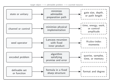
A complexity value is defined only after the target object selects an admissible family of paths or descriptions. Circuit length, physical control cost, Krylov spread, algorithmic resources, and sharp o-minimal format or degree answer different questions. The diagram is schematic and not to scale.
The semantic comparison is:
| Proposal | Target task | Admissible class and cost | Reference and tolerance | Regulator and continuum question | Operational or invariant content | Principal ambiguity |
|---|---|---|---|---|---|---|
| State circuit | Prepare ρtarget from ρreference | Declared local or Gaussian gates; size, depth, or path length | State reference; trace, fidelity, or covariance error | Fixed physical error as lattice spacing tends to zero | Preparation cost for the chosen gate model | Reference, stabilizer quotient, and gate penalties |
| Unitary circuit | Synthesize a unitary on a declared domain | Gates modulo permitted phases; size or depth | Identity or reference unitary; channel error | Energy-constrained domain and regulator matching | Implementation resource on that domain | Precision, generator normalization, and nonlocal gates |
| Channel complexity | Implement a completely positive channel | Allowed dilations, ancillas, and controls; circuit or control cost | Reference channel and channel distance | Energy constraint and environment model | Implementation resource after declared minimization | Dilation freedom and uncharged environment preparation |
| Krylov complexity | Evolve one seed operator in a Lanczos basis | Fixed Liouvillian and inner product; first Krylov-index moment | Seed and inner product fix the basis | Ultraviolet spectral tail and order of limits | Basis-relative operator spread | Seed, thermal inner product, and truncation |
| Computational complexity | Estimate or simulate an observable for an instance family | Algorithms satisfying a promise; time, queries, samples, or memory | Input encoding, error, and success probability | Family of regulated instances and scaling variable | Invariant only under stated reductions | Encoding and computational model |
| Sharp format and degree | Specify a definable set or function | Formulas in a fixed structure; filtration pair (F, D) | Presentation and reduction rules | Not a state-preparation continuum limit | Descriptive-geometric bounds | Choice of structure and presentation |
Where comparisons fail
Section titled “Where comparisons fail”The second figure groups the most common hidden changes of task. A quoted scaling is not robust until these changes have been tested or explicitly excluded.
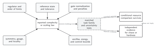
Reference sensitivity, gate nonuniqueness, regulator dependence, symmetry constraints, and unbounded controls are distinct failure modes. A link from complexity growth to chaos or computational hardness requires separate evidence after those controls. The diagram is schematic.
The thirteen pages
Section titled “The thirteen pages”- What Task Does Complexity Answer? supplies the comparison tuple and the four-way distinction among resource notions.
- Circuit Complexity in Quantum Field Theory defines regulated approximation by admissible circuits.
- Cost Geometry, Gate Sets, and Reference States develops Nielsen geometry and its normalization choices.
- State, Unitary, Channel, and Operator Complexity derives the inequivalent quotient freedoms of four targets.
- Gaussian-State Complexity turns covariance data into controlled solvable examples.
- Mixed-State, Purification, and Formation Complexity compares optimizations over spectra, bases, and ancillas.
- Interacting-Field Complexity states what perturbative and variational estimates actually control.
- Path-Integral and Euclidean Preparation Complexity separates Euclidean protocols from proposal-specific costs.
- Krylov and Operator-Growth Complexity derives the Lanczos-chain probability distribution.
- Complexity with Symmetry, Gauge, and Locality Constraints restricts admissible transformations before minimizing.
- Regulator Dependence and Continuum Complexity tests divergent terms and finite remainders across matched schemes.
- Operational Preparation Cost and Energy-Constrained Bounds connects abstract paths to bounded physical controls.
- Complexity, Chaos, and Computational Claims gives a claim matrix and explicit nonimplications.
Conventions and scope boundaries
Section titled “Conventions and scope boundaries”Circuit products act in their displayed time order; a page states whether its geometric convention is left- or right-invariant. Bosonic covariance matrices use canonical quadratures with the commutator normalization declared locally, while fermionic pages declare Majorana normalization. A cost carries its generator normalization and penalty schedule. Continuum claims compare a family of regulated tasks at fixed physical tolerance; subtracting a divergence without a permitted local cost and a matched reference does not create a universal observable.
Algorithms and tensor-network costs are developed in Volume 8, while physical operator dynamics and chaos diagnostics are developed in Volume 11. Holographic complexity proposals belong to Volume 15 and do not define generic QFT complexity here. A reproducible verification should compare matched finite-mode examples with identical regulators and cost conventions.
Review the chapter
Section titled “Review the chapter”Task translation. Two papers report different ultraviolet exponents for “the complexity of the vacuum.” Give a minimum comparison test.
Verification criteria
Match the target and reference families, gate generators and their normalization, locality and penalty rules, cost functional, error metric and tolerance, spatial volume, zero-mode treatment, regulator, and order of limits. If no controlled translation preserves these data, the exponents answer different questions.
Operational meaning. A geometric path has length and can be traversed in arbitrarily small parameter time. Why is not yet a laboratory duration?
Verification criteria
The path parameter is not physical time. A duration bound needs a control Hamiltonian, amplitude or energy limits, locality, bandwidth, and an implementation map from geometric generators to controls. Without those data, reparameterization changes duration while leaving fixed.
Nonimplication. Does rapidly growing Krylov complexity prove chaos?
Verification criteria
No. It proves spreading in the Lanczos basis fixed by a seed, inner product, and generator. A chaos claim also needs independent dynamical or spectral diagnostics, symmetry resolution, finite-size and regulator controls, and an argument excluding integrable or free counterexamples.
References
Section titled “References”- Binyamini, Gal, Dmitri Novikov, and Benny Zack. “Sharply o-Minimal Structures and Sharp Cellular Decomposition.” arXiv:2209.10972 (2022; revised 2024). Preprint.
- Jefferson, Ro, and Robert C. Myers. “Circuit Complexity in Quantum Field Theory.” Journal of High Energy Physics 10 (2017): 107. DOI. Open PDF.
- Nielsen, Michael A. “A Geometric Approach to Quantum Circuit Lower Bounds.” Quantum Information & Computation 6 (2006): 213–262. Open PDF.
- Parker, Daniel E., Xiangyu Cao, Alexander Avdoshkin, Thomas Scaffidi, and Ehud Altman. “A Universal Operator Growth Hypothesis.” Physical Review X 9 (2019): 041017. DOI. Open PDF.
Original QFT.org content:CC BY 4.0, unless an item supplies different terms. Third-party material retains its own terms.