Entropic Monotones in Two Dimensions

For the vacuum of a unitary Lorentz-invariant QFT in 1+1 dimensions, the entropy of one interval defines a dimensionless function that decreases with the interval’s proper length and equals the Virasoro central charge at conformal endpoints. The result is a theorem about a fixed vacuum interval family; finite temperature, a non-Lorentz-invariant scaling law, or the absence of a positive density-matrix framework removes a needed hypothesis.

Required background. Information measures along RG flows fixes what is varied, what is held fixed, and how endpoint claims are licensed.

Helpful background. Monotonicity and flow constraints supplies the CFT endpoint interpretation; strong subadditivity supplies the entropy inequality used below.

Before comparing curves, consult the chapter’s scale-separation map, comparison table, and independent validity gates. They separate a theorem about $R$ from cutoff refinement and from a change of state.

Normalize the interval c-function

Let $S(R)$ be the continuum vacuum entropy of an interval of proper length $R$. It is useful to keep two normalizations visible:

$$C(R)=R S'(R), \qquad c_E(R)=3C(R)=3R S'(R).$$

Casini and Huerta call $C$ the entropic $c$-function. This page uses $c_E$ so that the fixed-point value is the usual Virasoro central charge rather than one third of it. For an interval in the vacuum of a CFT on the infinite line,

$$S(R)=\frac{c}{3}\log\frac{R}{\epsilon}+s_0,$$

and therefore $C=c/3$ and $c_E=c$. The derivative removes the additive endpoint divergence $s_0$, but it must be taken only after $S(R)$ has a common continuum prescription.

Boosted diamonds turn strong subadditivity into a derivative

Use null coordinates $u=t-x$ and $v=t+x$. A causal diamond with null-coordinate widths $\Delta u$ and $\Delta v$ has interval proper length $\sqrt{\Delta u\,\Delta v}$. Choose boosted intervals $A$ and $B$ with diamond widths $(R,r)$ and $(r,R)$, where $0<r<R$. Both have proper length $\sqrt{rR}$; their overlap $Y$ has length $r$, while the causal completion $XYZ$ of their union has length $R$. Strong subadditivity and causal-domain invariance then give

$$2S(\sqrt{rR})\ge S(r)+S(R).$$

The figure encodes precisely this product-of-null-widths relation; inspect how intersection and causal completion stay in the same one-interval family.

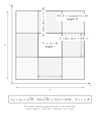
Null-coordinate geometry behind the 1+1-dimensional proof. For $0<r<R$, boosted intervals $A$ and $B$ have equal proper length $\sqrt{rR}$, their overlap $Y$ has length $r$, and the causal completion $XYZ$ has length $R$, so strong subadditivity gives $2S(\sqrt{rR})\ge S(r)+S(R)$. The state is the Lorentz-invariant vacuum and all four entropies use one regulator or algebraic prescription. Schematic; not to scale.

Set $R=r+\delta$ and expand through order $\delta^2$. Assuming the continuum function is twice differentiable produces

$$rS''(r)+S'(r)\le0,$$

or, after renaming $r$ as $R$,

$$\frac{dc_E}{dR} =3\bigl[S'(R)+RS''(R)\bigr]\le0.$$

The finite inequality, its infinitesimal limit, and the source normalization $C=RS'$ are derived in Casini and Huerta 2007, pp. 7033–7035, eqs. (8)–(16). Ordinary nested intervals on one equal-time slice do not reproduce the crossed null widths and hence do not give this derivative inequality.

The conclusion is

$$c_{\rm UV}=\lim_{R\to0}c_E(R) \ge \lim_{R\to\infty}c_E(R)=c_{\rm IR},$$

provided the limits reach CFTs. For a trivial gapped infrared theory, the interval entropy saturates and $c_E\to0$. Equality of the entropy inequality over a scale range says that $RS'$ is constant on that range; identifying the whole theory as a fixed point requires the usual additional QFT assumptions.

Massive free fields give an analytic benchmark

For one free massive Dirac field or one real massive scalar, put $t=mR$. In the source convention the functions are $C_D(t)$ and $C_S(t)$; multiplying by three gives the normalization used here. The leading controlled limits are Casini and Huerta 2007, pp. 7034–7035, eqs. (15)–(16):

Field and regime	Page-normalized result	Quantitative check
Dirac, $t\ll1$	$c_E^D(t)=1-t^2\log^2t+O(t^2\lvert\log t\rvert)$	$c_E^D(0)=1$; the displayed correction decreases for sufficiently small $t$
Scalar, $t\ll1$	$c_E^S(t)=1+3/(2\log t)+O(\log^{-2}t)$	$c_E^S(0)=1$, approached only logarithmically because of the zero mode
Dirac, $t\gg1$	$c_E^D(t)=\tfrac32 tK_1(2t)+o(tK_1(2t))$	$c_E^D(\infty)=0$
Scalar, $t\gg1$	$c_E^S(t)=\tfrac34 tK_1(2t)+o(tK_1(2t))$	$c_E^S(\infty)=0$

Here $K_\nu$ is a modified Bessel function. The large-$t$ derivative is manifestly negative because

$$\frac{d}{dt}\bigl[tK_1(2t)\bigr]=-2tK_0(2t)<0.$$

The scalar’s slow ultraviolet approach is a useful adversary for numerical work: at leading order, $t=10^{-6}$ gives $1+3/(2\log t)\simeq0.89143$, not a value visually indistinguishable from $1$. This number is an asymptotic estimate, not a replacement for the exact Painlevé solution; its uncertainty is the displayed $O(\log^{-2}t)$ truncation. The integral equations and full scalar–Dirac comparison are given in Casini and Huerta 2009, §§ 3.1.1–3.1.3, especially fig. 9 and eq. (154).

A reproducible finite-grid calculation should declare the lattice spacing $a$, total length $L$, interval endpoints, and mass in lattice units; hold $t=mR$ fixed while sending $a/R\to0$ and $R/L\to0$; fit $S$ with its covariance rather than differencing independent rounded values; and quote the spread under at least two fit windows and two refinements. The exact endpoint values above have no numerical uncertainty. Every finite-$t$ lattice value carries discretization, finite-volume, fit-covariance, and asymptotic-truncation errors, which must be reported separately.

Finite temperature is an exact failure test

For a CFT thermal state on the infinite line at inverse temperature $\beta$,

$$S_\beta(R)=\frac{c}{3} \log\!\left[ \frac{\beta}{\pi\epsilon} \sinh\!\left(\frac{\pi R}{\beta}\right) \right]+s_\beta,$$

as derived in Calabrese and Cardy 2004, eq. (3) and § III. With $x=\pi R/\beta$,

$$c_E^{(\beta)}(R)=c\,x\coth x,$$

and

$$\frac{dc_E^{(\beta)}}{dR} =\frac{c\pi}{\beta} \left(\coth x-x\,\operatorname{csch}^2x\right)>0 \qquad (R>0).$$

At $x=1$, $c_E^{(\beta)}/c=\coth1\simeq1.31304$ and $(\beta/\pi c)\,\frac{d c_E^{(\beta)}}{dR}\simeq0.588974$; the last shown digits are rounded, with error below $5\times10^{-6}$. This is not a counterexample to the theorem. The thermal state is not the Lorentz-invariant vacuum, and the additional scale $\beta$ invalidates the step that assigns entropy using only proper length. The strongest surviving statement is the exact thermal formula and its extensive large-$R$ limit, not vacuum $c$-monotonicity.

A Lifshitz theory fails at the same geometric step because boosts are not symmetries. Strong subadditivity itself remains true for every positive density matrix; the issue in a nonunitary QFT is that the positive Hilbert-space and density-matrix framework needed to invoke it may be absent.

Common pitfalls

Importing the source curve without its normalization. The primary free-field papers plot $C=RS'$, whose CFT value is $c/3$. Multiply by three before comparing with the $c_E$ used here.

Differentiating before taking a common continuum limit. A coarse grid or independently fitted entropies can manufacture a small upward step. Refine the regulator at fixed $mR$ and propagate correlated errors through the derivative.

Calling a thermal interval a failed vacuum theorem. The exact thermal derivative is positive because the state introduces $\beta$ and eventually extensive entropy. It tests the scope of the proof rather than contradicting it.

Exercises

1. Starting from $2S(\sqrt{rR})\ge S(r)+S(R)$, set $R=r+\delta$ and derive the differential inequality through order $\delta^2$.

Solution

The geometric mean expands as

$$\sqrt{r(r+\delta)} =r+\frac{\delta}{2}-\frac{\delta^2}{8r}+O(\delta^3).$$

Taylor expansion gives

$$2S(\sqrt{rR}) =2S(r)+\delta S'(r) +\frac{\delta^2}{4}S''(r) -\frac{\delta^2}{4r}S'(r)+O(\delta^3),$$

whereas $S(r)+S(r+\delta)=2S(r)+\delta S'(r)+\delta^2S''(r)/2+O(\delta^3)$. Subtracting the right-hand side and requiring the coefficient of $\delta^2$ to be nonnegative yields $-S''/4-S'/(4r)\ge0$, or $rS''+S'\le0$.

2. Use the leading scalar ultraviolet expression to show both that $c_E^S(t)\to1$ and that its approach is monotone for sufficiently small positive $t$.

Solution

As $t\to0^+$, $\log t\to-\infty$, so $3/(2\log t)\to0^-$ and $c_E^S\to1$ from below. Differentiating the displayed leading term gives

$$\frac{dc_E^S}{dt} =-\frac{3}{2t\log^2t}<0.$$

The omitted $O(\log^{-2}t)$ terms do not change this conclusion once $t$ is sufficiently small; a finite-$t$ numerical claim must check them rather than treating the leading expression as exact.

3. Prove that the finite-temperature derivative is positive without using a plot.

Solution

For $x>0$,

$$\coth x-x\operatorname{csch}^2x =\frac{\sinh x\cosh x-x}{\sinh^2x}.$$

The numerator is positive because $\sinh x\cosh x=\tfrac12\sinh(2x)>x$ for $x>0$. Hence $dc_E^{(\beta)}/dR>0$. At large $x$, $x\coth x\sim x$, so $S_\beta'(R)\to\pi c/(3\beta)$, the thermal entropy density.

References

• Calabrese, Pasquale, and John Cardy. “Entanglement Entropy and Quantum Field Theory.” Journal of Statistical Mechanics: Theory and Experiment 2004, no. 6 (2004): P06002. DOI. Open PDF.
• Casini, Horacio, and Marina Huerta. “A c-Theorem for the Entanglement Entropy.” Journal of Physics A: Mathematical and Theoretical 40 (2007): 7031–7036. DOI. Open PDF.
• Casini, Horacio, and Marina Huerta. “Entanglement Entropy in Free Quantum Field Theory.” Journal of Physics A: Mathematical and Theoretical 42 (2009): 504007. DOI. Open PDF.