Corners, Cusps, and Defect Data

Corners are a singular limit of entangling-surface geometry. At a three-dimensional conformal fixed point they add a universal angle-dependent logarithm that is absent for a smooth curve. A generic massive three-dimensional QFT need not have the same scale-independent function: the CFT or ultraviolet-fixed-point limit, the interior-angle convention, and the physical regulator metric must all be stated. This page separates exact endpoint theorems, finite-$n$ defect conjectures, direct free-field results, and a reproducible interpolation benchmark so that agreement between them is never mistaken for one kind of proof.

Required background. Use Universal Terms and Entangling-Surface Geometry to separate the logarithm from local perimeter terms, and Shape Dependence and Entanglement Variations to understand why the smooth harmonic expansion ceases to converge at a cusp. Helpful background. Twist and replica defects supplies the replicated theory and the defect operators used below.

The three-dimensional corner function

For one corner of interior opening angle $0<\theta<2\pi$ in the vacuum of a three-dimensional CFT,

$$S^{\mathcal R}(A) =\alpha_{\mathcal R}\frac{L}{\epsilon} -a(\theta)\log\frac{L}{\epsilon} +O(1).$$

Here $\mathcal R$ denotes the UV regulator, $\epsilon$ its physical short-distance scale, and $L$ a macroscopic scale used to separate the corner from other geometric features. The angle $\theta$ is measured with the continuum physical metric, not merely with lattice coordinates. For a polygon, the logarithmic coefficient is the sum of the functions for well-separated vertices. The perimeter coefficient and finite term depend on the regulator, but $a(\theta)$ is a continuum CFT datum after the physical angle and subtraction are fixed Casini and Huerta 2007, §1, eqs. (4)–(7), preprint pp. 1–2, PDF.

For a pure state with a matched algebra for $A$ and its complement, complementarity gives

$$a(\theta)=a(2\pi-\theta).$$

This symmetry is not automatic for a mixed state or for mismatched algebra choices. On $0<\theta\le\pi$, positivity and strong subadditivity imply

$$a(\theta)\ge0, \qquad a'(\theta)\le0, \qquad a'(\theta)+\sin\theta\,a''(\theta)\ge0.$$

The last inequality also implies convexity in this interval. These constraints and their stronger lower bound are derived in Bueno and Witczak-Krempa 2016, §II, eqs. (II.1)–(II.2), pp. 3–5, PDF.

Two asymptotic coefficients organize the full angular function:

$$a(\theta) =\sigma(\pi-\theta)^2+O((\pi-\theta)^4) \quad(\theta\to\pi), \qquad a(\theta)=\frac{\kappa}{\theta}+O(1) \quad(\theta\to0).$$

The figure relates the opening angle to these two limits. Inspect the different geometric neighborhoods: a nearly straight line measures $\sigma$, whereas a thin wedge measures $\kappa$. The solid and dashed curves preview the reproducible smooth–sharp benchmark developed below: they share the same exact $\sigma$ but separate toward small angle because their $\kappa$ values differ.

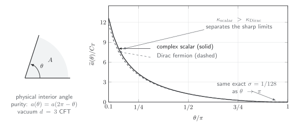
For one corner in a vacuum $d=3$ CFT, purity relates complementary angles. The quantitative panel evaluates the Helmes et al. smooth–sharp ansatz from published $M=8$ complex-scalar and $M=7$ Dirac inputs, normalized by their common $C_T=3/(16\pi^2)$. Both approach $\sigma(\pi-\theta)^2$ with $\sigma=1/128$, while $\kappa_{\rm scalar}=0.0794>\kappa_{\rm Dirac}=0.0722$ separates the sharp limits. The wedge is schematic; the plotted curves are a high-precision interpolation, not direct solutions of the cut-sphere equations.

The chapter structure map locates this singular geometric datum, while the canonical comparison table keeps it distinct from mixed-state and multipartite measures.

Stress-tensor and replica-defect data

Normalize the Euclidean stress tensor by

$$\langle T_{\mu\nu}(x)T_{\rho\sigma}(0)\rangle =\frac{C_T}{\lvert x\rvert^6}\mathcal I_{\mu\nu,\rho\sigma}(x).$$

Writing

$$I_{\mu\nu}(x)=\delta_{\mu\nu}-2\frac{x_\mu x_\nu}{x^2}, \qquad \mathcal I_{\mu\nu,\rho\sigma} =\frac12\left(I_{\mu\rho}I_{\nu\sigma}+I_{\mu\sigma}I_{\nu\rho}\right) -\frac13\delta_{\mu\nu}\delta_{\rho\sigma}$$

fixes the normalization on which every numerical relation below depends. Unitarity gives $C_T>0$. Then every unitary $d=3$ CFT obeys the smooth-corner relation

$$\sigma=\frac{\pi^2}{24}C_T.$$

It follows from the universal separated-point shape kernel Faulkner, Leigh, and Parrikar 2016, §4.1, eq. (107), p. 22, PDF. The full $a(\theta)$ is not fixed by $C_T$; two theories can share $C_T$ and $\sigma$ while differing at finite angle or in $\kappa$.

For Rényi entropy, write

$$S_n^{\mathcal R}(A) =B_{n,\mathcal R}\frac{L}{\epsilon} -a_n(\theta)\log\frac{L}{\epsilon}+O(1), \qquad a_n(\theta)=\sigma_n(\pi-\theta)^2+\cdots.$$

The replica twist line is a conformal defect. If $a$ labels the two directions transverse to the line and $y$ runs along it, broken transverse translation defines the displacement operator through the Ward identity

$$\sum_{m=1}^{n}\partial_\mu T_{(m)}^{\mu a}(x) =\delta_\Sigma(x)D^a(y).$$

Its normalization is therefore fixed rather than freely rescalable. Conformal symmetry gives the separated defect correlator

$$\langle D^a(y)D^b(0)\rangle_n =\frac{C_D(n)\delta^{ab}}{\lvert y\rvert^{2(d-1)}}.$$

The datum $C_D(n)$ controls the nonlocal second-order response to a shape deformation; coincident insertions can also produce regulator-dependent contact terms. The twist scaling dimension $h_n$ is a different datum, fixed by the stress-tensor one-point function around the defect Bianchi et al. 2016, §2, eqs. (2.8)–(2.15), pp. 6–8, PDF.

The logical status of the relations is important:

• Theorem at $n=1$. The entanglement limit of the separated shape response is fixed by $C_T$, giving $\sigma/C_T=\pi^2/24$.

• Finite-$n$ proposal. The constraint

  $$C_D(n)=d\,\Gamma\!\left(\frac{d+1}{2}\right) \left(\frac{2}{\sqrt\pi}\right)^{d-1}h_n$$

  holds infinitesimally around $n=1$ and in important examples, but fails as a universal identity for arbitrary $n$ and every CFT.

• Corner consequence. In three dimensions, the relation

  $$\sigma_n=\frac{h_n}{\pi(n-1)}$$

  between the smooth Rényi coefficient and $h_n$ has compelling free-field and holographic checks, but it is a conjecture for a completely general CFT Bueno, Myers, and Witczak-Krempa 2015, §1.1, eq. (1.6), pp. 2–4, and §3.2, pp. 12–15, PDF. At $n\to1$, its limit reduces to the proven $\sigma/C_T$ relation.

An entanglement corner is also not automatically a Wilson-line cusp. The former belongs to the replica twist defect and depends on the state and entropy index; the latter belongs to a chosen line operator and has its own representation and couplings. In specified supersymmetric classes, selected displacement or Bremsstrahlung coefficients can be related. That restricted coefficient relation does not identify the two full angular functions Bianchi et al. 2016, §4.2, pp. 15–16, PDF. The general defect normalization and its contact terms are developed on The displacement operator and defect Ward identities.

Free-field angular benchmark

Casini and Huerta reduced the scalar corner to Green functions on a cut sphere and checked the result on a square lattice 2007, §2 and Appendix B, PDF. Casini, Huerta, and Leitao performed the corresponding Dirac calculation and tabulated both functions 2009, §IV and Table 1, pp. 8–9, PDF. These are direct continuum calculations. They give, for a complex scalar—two independent real scalars—and a two-component Dirac fermion,

Quantity	Complex scalar	Dirac fermion
Direct $a(\pi/2)$	0.02366	0.02329
Direct $a(3\pi/4)$	0.005040	0.005022
Exact $\sigma$	$1/128$	$1/128$
Sharp input $\kappa$	0.0794	0.0722

Both theories have $C_T=3/(16\pi^2)$, so the exact smooth coefficient obeys

$$\frac{\sigma}{C_T} =\frac{1/128}{3/(16\pi^2)} =\frac{\pi^2}{24}.$$

The different $\kappa$ values and the small finite-angle difference show concretely why $C_T$ does not determine the entire curve.

A reproducible smooth–sharp interpolation

To make the angular comparison inspectable, the accompanying generator evaluates the high-precision interpolation of Helmes et al. rather than pretending to rerun the original cut-sphere solvers. With $M=8$ for the complex scalar and $M=7$ for the Dirac fermion,

$$\widetilde a(\theta) =\sum_{p=1}^{M}\sigma^{(p-1)}(\theta-\pi)^{2p} +\frac{2\kappa}{\pi^{2M+1}} \frac{(\theta-\pi)^{2(M+1)}}{\theta(2\pi-\theta)}.$$

The first term uses the published smooth coefficients, while the rational completion builds in the sharp limit. It is a high-precision ansatz, not an exact formula for the full curve Helmes et al. 2016, §III.D, eq. (22), pp. 5–6, Tables I–IV, pp. 10 and 13–14, PDF.

The generated values below reproduce the source tables. Each entry is “ansatz / independent lattice extrapolation”; the lattice calculation used a numerical linked-cluster expansion for the boson and a finite-size correlation-matrix method for the fermion.

Physical angle	Complex scalar	Dirac fermion
$\arctan(1/2)$	0.15575 / 0.154	0.14649 / 0.147
$\pi/4$	0.08102 / 0.0809	0.07760 / 0.0777
$\arctan 2$	0.04819 / 0.0483	0.04679 / 0.0466
$\pi/2$	0.02367 / 0.0236	0.02329 / 0.02329
$\pi-\arctan 2$	0.01051 / 0.0105	0.01043 / 0.0106
$3\pi/4$	0.005040 / 0.00507	0.005022 / 0.0049
$\pi-\arctan(1/2)$	0.001705 / 0.00170	0.001703 / 0.002

The structured JSON record preserves every coefficient, source locator, endpoint fit, rounded lattice comparison, and limitation. The complete plotting CSV contains forty angles from $\theta/\pi=0.025$ to $1$.

Endpoint fits and what they establish

The generator fits

$$\frac{\widetilde a(\pi-\delta)}{\delta^2} =\sigma_{\rm fit}+b_2\delta^2+b_4\delta^4, \qquad \theta\widetilde a(\theta) =\kappa_{\rm fit}+c_1\theta+c_2\theta^2$$

over three nested windows. The angular variables are in radians. The narrowest window, $\delta_{\max}=\theta_{\max}=0.1$, gives

Theory	$\sigma_{\rm fit}$	input $\sigma$	$\kappa_{\rm fit}$	input $\kappa$
Complex scalar	0.00781250000016	0.0078125	0.07940124	0.0794
Dirac fermion	0.00781250000015	0.0078125	0.07220052	0.0722

Across the three windows the $\sigma$ intercept spreads are below $7.0\times10^{-10}$, while the $\kappa$ spreads are $5.5\times10^{-5}$ for the scalar and $3.0\times10^{-5}$ for the fermion. Omitting the last supplied smooth coefficient changes the seven tabulated ansatz values by at most $9.7\times10^{-5}$ relatively for the scalar and $1.7\times10^{-5}$ for the fermion.

Those numbers are implementation and interpolation-stability diagnostics, not confidence intervals on the exact continuum functions: $\sigma$ and $\kappa$ were inputs to the ansatz. The independent lattice columns provide the external check. Their source reports robust displayed digits under fit-window variation and estimates systematic uncertainty at roughly the third significant digit, without claiming strict confidence intervals. A new direct computation would still have to vary the cut-sphere quadrature or lattice spacing itself.

Adversarial anisotropic-lattice test

Let the lattice spacings be $a_x$ and $a_y$. A coordinate displacement $(v_x,v_y)$ represents the physical vector $(a_xv_x,a_yv_y)$. The axis-aligned rays $(1,0)$ and $(0,1)$ remain physically orthogonal. The coordinate-orthogonal diagonal rays $(1,1)$ and $(-1,1)$ instead have

$$\cos\theta_{\rm phys} =\frac{a_y^2-a_x^2}{a_x^2+a_y^2}.$$

For $a_x=2a_y$, the nominal diagonal “right angle” is actually

$$\theta_{\rm phys}=\arccos(-3/5)\approx126.87^\circ.$$

Thus rotating a fixed coordinate corner at fixed anisotropy changes the continuum geometry by $36.87^\circ$; an orientation-dependent fitted $a$ is then expected and is not evidence against universality. Calibrate the physical metric first, define the same $\theta_{\rm phys}$ in each orientation, and fit

$$\Delta_h(\theta) =a_h(\theta,0)-a_h(\theta,\pi/4) =\Delta_0+c h^\omega+\cdots.$$

Here $h$ is the physical refinement scale after metric calibration and $\omega>0$ is the leading correction exponent used in the continuum extrapolation. If the continuum fixed point restores rotational invariance, a valid isotropic extraction requires $\Delta_0$ to agree with zero within the refinement and fit-window uncertainty. Without restored isotropy, zero is not the expected target. If the raw coordinate angle is held fixed at $a_x/a_y=2$, an $O(1)$ intercept can survive because the two calculations are different physical wedges. The validity map makes this regulator-geometry matching requirement explicit.

Higher-dimensional cones and cusps can generate additional curvature invariants or powers of logarithms. The $d=3$ function above must not be transferred across spacetime dimension or singularity class without a new derivation.

Common pitfalls

Calling the corner coefficient universal in any three-dimensional QFT. Scale independence follows at a conformal fixed point. A mass scale introduces crossover functions and can spoil the CFT form.

Using purity symmetry for a mixed state. The equality $a(\theta)=a(2\pi-\theta)$ compares complementary regions in a pure state with matched algebras. State those hypotheses.

Comparing coordinate angles on an anisotropic regulator. Universality refers to the physical continuum angle. Calibrate velocities or spacings before rotating the corner.

Treating an endpoint round trip as an independent measurement. The smooth–sharp ansatz contains $\sigma$ and $\kappa$ as inputs. Fitting its generated curve back to those endpoints checks the implementation and window stability, not the underlying continuum calculation.

Exercises

1. Suppose $a(\theta)=\sigma\delta^2+\tau\delta^4+O(\delta^6)$ with $\delta=\pi-\theta$. Use the strong-subadditivity inequality to constrain $\tau$.

Solution

Since $a'=-2\sigma\delta-4\tau\delta^3+O(\delta^5)$, $a''=2\sigma+12\tau\delta^2+O(\delta^4)$, and $\sin\theta=\sin\delta=\delta-\delta^3/6+O(\delta^5)$,

$$a'+\sin\theta\,a'' =\left(8\tau-\frac{\sigma}{3}\right)\delta^3+O(\delta^5).$$

Nonnegativity for sufficiently small positive $\delta$ gives $\tau\ge\sigma/24$.

2. Verify the smooth-limit relation for the complex scalar and Dirac fermion in the table, and explain why it does not predict their sharp limits.

Solution

For either theory, $C_T=3/(16\pi^2)$ and $\sigma=1/128$. Hence

$$\sigma/C_T=(1/128)(16\pi^2/3)=\pi^2/24.$$

The sharp coefficients are nevertheless $0.0794$ and $0.0722$. The smooth relation fixes only the quadratic Taylor coefficient at $\theta=\pi$; it contains no theorem determining the entire function or its opposite endpoint.

3. On a lattice with $a_x=2a_y$, compute the physical angle between the diagonal rays $(1,1)$ and $(-1,1)$. What continuum test removes the resulting false orientation dependence?

Solution

The physical rays are $(2a_y,a_y)$ and $(-2a_y,a_y)$. Their dot product is $-3a_y^2$, and each has norm $\sqrt5a_y$. Therefore $\cos\theta=-3/5$ and $\theta\approx126.87^\circ$, not $90^\circ$.

One must redraw the rays so that their angle in the calibrated physical metric is the same in both orientations, or take the isotropic limit $a_x/a_y\to1$. After that correction, extrapolate the orientation difference $\Delta_h$ and require its continuum intercept to be compatible with zero.

4. Assume in $d=3$ that the proposed finite-$n$ relation between displacement and twist data holds. Combine it with the proposed smooth-corner relation to express $C_D(n)$ in terms of $\sigma_n$. Which part of the argument remains valid without that finite-$n$ assumption?

Solution

For $d=3$, the proposed defect relation becomes

$$C_D(n) =3\Gamma(2)\left(\frac{2}{\sqrt\pi}\right)^2h_n =\frac{12}{\pi}h_n.$$

Using $\sigma_n=h_n/[\pi(n-1)]$ then gives

$$C_D(n)=12(n-1)\sigma_n.$$

This equality is conditional at general $n$: the proposed $C_D$–$h_n$ constraint is not a theorem for every CFT, and neither is the general finite-$n$ corner formula. In the entanglement limit $n\to1$, the first derivative of $C_D(n)$ is fixed by $C_T$ and the resulting relation $\sigma/C_T=\pi^2/24$ is universal.

References

• Bianchi, Lorenzo, Marco Meineri, Robert C. Myers, and Michael Smolkin. “Rényi Entropy and Conformal Defects.” Journal of High Energy Physics 2016, no. 07 (2016): 076. DOI. Open PDF.
• Bueno, Pablo, Robert C. Myers, and William Witczak-Krempa. “Universal Corner Entanglement from Twist Operators.” Journal of High Energy Physics 2015, no. 09 (2015): 091. DOI. Open PDF.
• Bueno, Pablo, and William Witczak-Krempa. “Bounds on Corner Entanglement in Quantum Critical States.” Physical Review B 93, no. 4 (2016): 045131. DOI. Open PDF.
• Casini, Horacio, and Marina Huerta. “Universal Terms for the Entanglement Entropy in 2+1 Dimensions.” Nuclear Physics B 764 (2007): 183–201. DOI. Open PDF.
• Casini, Horacio, Marina Huerta, and Leonardo Leitao. “Entanglement Entropy for a Dirac Fermion in Three Dimensions: Vertex Contribution.” Nuclear Physics B 814, no. 3 (2009): 594–609. DOI. Open PDF.
• Faulkner, Thomas, Robert G. Leigh, and Onkar Parrikar. “Shape Dependence of Entanglement Entropy in Conformal Field Theories.” Journal of High Energy Physics 2016, no. 04 (2016): 088. DOI. Open PDF.
• Helmes, Johannes, Lauren E. Hayward Sierens, Anushya Chandran, William Witczak-Krempa, and Roger G. Melko. “Universal Corner Entanglement of Dirac Fermions and Gapless Bosons from the Continuum to the Lattice.” Physical Review B 94, no. 12 (2016): 125142. DOI. Open PDF.