Modular Berry Transport and Holonomy

Modular Berry transport compares an isolated modular spectral sector along a smooth family of states or regions. The comparison is not unique inside a degenerate sector: every change of frame that commutes with the modular generator is a zero-mode gauge transformation. Consequently, a closed-path matrix is meaningful only up to conjugation; its conjugacy class, eigenvalues, and class functions are the observables.

Required background. Modular spectra and spectral measures supply spectral projectors, direct-integral language, and the distinction between point and continuous spectrum.

Helpful background. State perturbations and susceptibility supply differentiable faithful families and their regulator controls.

The chapter’s differentiable-family map locates projected modular transport alongside state and shape response, while the independent validity gates separate the obligations a regulated holonomy must pass. In particular, a successful finite-dimensional calculation does not by itself settle the continuum spectral or algebra-identification gates.

Zero modes and constant-rank spectral blocks

Begin with a faithful finite regulator and a smooth Hermitian modular generator

$$K(\lambda)=U(\lambda)D(\lambda)U(\lambda)^\dagger.$$

The relevant zero modes are operators in the kernel of the modular Liouvillian

$$\mathcal L_K(X):=[K,X].$$

If $K=\sum_\alpha \kappa_\alpha P_\alpha$, where the sum is over distinct eigenvalues, then

$$P_0^K(X)=\sum_\alpha P_\alpha X P_\alpha.$$

Thus a multiplicity-$m_\alpha$ eigenspace contributes the full matrix algebra $M_{m_\alpha}$, not merely $m_\alpha$ independent phases. Equivalently,

$$P_0^K(X)=\lim_{T\to\infty}\frac{1}{2T} \int_{-T}^{T}e^{isK}Xe^{-isK}\,ds$$

in the finite model, and in a continuum setting only when the mean ergodic limit exists in the stated topology. “Zero mode” here means zero Liouvillian frequency; it does not mean a zero eigenvalue of $K$.

To transport one cluster, choose a spectral projector $P(\lambda)$ of fixed rank $m$ separated from the rest of the spectrum by a gap $\gamma>0$. Smoothness of the corresponding Riesz projector follows while that contour remains in the resolvent set Kato 1952, pp. 323–327. Internal eigenvalue coincidences are harmless if the whole cluster is retained. A crossing through the cluster boundary, or any closure of $\gamma$, removes the hypothesis needed for this connection.

Connection, convention, and holonomy

Let $Q(\lambda):\mathbb C^m\to\mathcal H$ be an orthonormal frame for the chosen block, so $Q^\dagger Q=\mathbf 1_m$ and $QQ^\dagger=P$. We use the anti-Hermitian frame connection

$$\mathcal A:=Q^\dagger dQ, \qquad \mathcal A^\dagger=-\mathcal A,$$

and orient parallel transport along increasing path parameter by

$$W[C]:=\mathcal P\exp\!\left(-\oint_C\mathcal A\right).$$

For a complete diagonalizer, $P_0^D(U^\dagger dU)$ is the direct sum of these block connections. The superscript matters: $U^\dagger dU$ is in the $D$-frame, whereas $P_0^K$ acts in the physical $K$-frame. This separates commuting frame motion from horizontal motion. The modular construction likewise defines zero modes by commutation with $H_{\rm mod}$ and treats their local frame freedom as gauge Czech et al. 2018, pp. 2–3, eqs. (4) and (12)–(13).

Under a change of block frame $Q\mapsto Qg$, $g(\lambda)\in U(m)$,

$$\mathcal A\mapsto g^\dagger\mathcal A g+g^\dagger dg, \qquad W[C]\mapsto g(\lambda_0)^\dagger W[C]g(\lambda_0)$$

for a single-valued frame around a closed loop based at $\lambda_0$. This is the Wilczek–Zee non-Abelian connection for a degenerate block Wilczek and Zee 1984, pp. 2111–2113. The curvature is

$$\mathcal F=d\mathcal A+\mathcal A\wedge\mathcal A =\frac12\mathcal F_{ij}\,d\lambda^i\wedge d\lambda^j.$$

For a sufficiently small loop of linear size $\ell$ in a smooth patch, define its antisymmetric area tensor by $\Sigma^{ij}=\int_\Sigma d\lambda^i\wedge d\lambda^j$. Then

$$W=\mathbf1-\frac12\mathcal F_{ij}\Sigma^{ij}+O(\ell^3).$$

A Gaussian modular eigenspace around a loop

Here is a reproducible regulated QFT application. Take four fermionic wave-packet modes, grouped as a two-level orbital index with two identical flavors, and the faithful Gaussian state

$$\rho(\boldsymbol n)=Z^{-1} \exp\!\left[-c^\dagger h(\boldsymbol n)c\right], \qquad h(\boldsymbol n)=\varepsilon\,\boldsymbol n\cdot\boldsymbol\sigma\otimes\mathbf1_2, \qquad \varepsilon>0.$$

For a fermionic Gaussian state the one-particle correlation matrix is $C=(\mathbf1+e^h)^{-1}$ Peschel 2003, pp. L205–L207, eqs. (3)–(7). The one-particle eigenvalues $\pm\varepsilon$ are separated by $2\varepsilon$ and each has multiplicity two. We transport the $+\varepsilon$ block along the latitude

$$\boldsymbol n(\phi) =(\sin\theta_0\cos\phi,\sin\theta_0\sin\phi,\cos\theta_0), \qquad 0\le\phi\le2\pi.$$

Choose

$$Q(\phi)= \begin{pmatrix} \cos(\theta_0/2)\\ e^{i\phi}\sin(\theta_0/2) \end{pmatrix}\otimes\mathbf1_2.$$

The figure separates the spectral condition from the gauge statement. Inspect the nonzero $2\varepsilon$ gap all along the latitude, then follow how changing the $U(2)$ frame conjugates the closed-loop Wilson map without changing its spectrum.

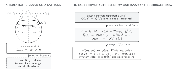
Along $\boldsymbol n(\phi)$ at $\theta_0=\pi/3$, the $+\varepsilon$ one-particle block has rank two and remains separated from the $-\varepsilon$ block by $2\varepsilon>0$. A periodic eigenframe $Q$ defines the horizontal frame $\widetilde Q=QW$, and a periodic frame change conjugates $W[C]$, so only conjugacy data are frame independent. When $\varepsilon\to0$, the former rank-two projector is no longer intrinsically selected; transporting a chosen limiting subbundle would require extra structure. The diagram is schematic and not to scale.

Then

$$\mathcal A_\phi =i\sin^2\!\left(\frac{\theta_0}{2}\right)\mathbf1_2, \qquad W[C]=e^{-i\pi(1-\cos\theta_0)}\mathbf1_2.$$

At $\theta_0=\pi/3$, the solid angle is $\Omega=\pi$ and $W=-i\mathbf1_2$. This is a holonomy of an isolated one-particle modular block; the induced many-body Gaussian transport follows by second quantization, but it should not be confused with a finite-rank eigenspace of a continuum local-QFT modular operator.

A basis-independent discretization uses overlap matrices $M_j=Q(\phi_j)^\dagger Q(\phi_{j+1})$ and their polar unitaries $L_j=M_j(M_j^\dagger M_j)^{-1/2}$. The links must be invertible, which holds for a sufficiently fine mesh on this smooth constant-rank loop. With $\phi_j=2\pi j/N$, define $W_N=L_{N-1}^\dagger\cdots L_0^\dagger$. For this loop,

$$M_j=\left[ \cos^2\!\frac{\theta_0}{2} +e^{2\pi i/N}\sin^2\!\frac{\theta_0}{2} \right]\mathbf1_2.$$

The convergence check at $\theta_0=\pi/3$ is:

$N$	$\lVert W_N-(-i\mathbf1_2)\rVert_2$
8	$6.295\times10^{-2}$
16	$1.529\times10^{-2}$
32	$3.794\times10^{-3}$
64	$9.468\times10^{-4}$

The controls are the spectral gap $2\varepsilon$, fixed rank two, loop orientation, polar-decomposition convention, and step number $N$. The observed factor-of-four reduction under $N\mapsto2N$ is the expected $O(N^{-2})$ error for this smooth symmetric loop.

Adversarial zero-mode-frame test

Replace the frame at every sampled point by $Q_jg_j$ with arbitrary $g_j\in U(2)$ and $g_N=g_0$. Each link transforms as

$$L_j\mapsto g_j^\dagger L_jg_{j+1},$$

so the product telescopes:

$$W_N\mapsto g_0^\dagger W_Ng_0.$$

For a generic noncentral holonomy, individual entries change while the eigenvalues, $\operatorname{tr}W_N$, and $\det W_N$ do not. In the latitude benchmark above, $W_N$ is proportional to $\mathbf1_2$, so conjugation leaves even its entries unchanged; the calculation verifies the covariance law but is not an entrywise gauge-sensitivity test. A result that changes by more than conjugation under the $g_j$ test is basis contamination, not modular holonomy. If $g_N\ne g_0$, one has changed the endpoint identification; the missing transition function must be included before comparing closed-loop answers.

Continuum and region-family limits

For a family of regions, the local algebras differ. One must first give embeddings or isomorphisms into a common reference algebra; changing those identifications changes the connection. In local QFT the modular spectrum is commonly continuous, so an eigenframe may be replaced by a direct integral, a spectral window, or an ergodic projection defined only in a weak topology. The inverse of $\operatorname{ad}_K$ on the nonzero-frequency sector also requires a named domain.

A continuum claim must therefore state the algebra identification, spectral window or projector, topology of $P_0$, constant-rank or gap condition, common domain, path-discretization convergence, and regulator order. The special geometric interpretation in vacuum two-dimensional CFT and AdS$_3$ is established under conformal and holographic hypotheses Czech et al. 2018, pp. 3–5; it is not a theorem that generic modular holonomy equals spacetime curvature.

Common pitfalls

Calling an eigenvalue of $K$ a zero mode. The zero-mode projector acts on operators and selects the kernel of $[K,\cdot]$. Degeneracy therefore enlarges the gauge algebra.

Mixing the physical and diagonal frames. Apply $P_0^D$ to $U^\dagger dU$, or conjugate both objects back to the $K$-frame. Mixing them produces a frame-dependent formula.

Continuing through a closing gap. Internal degeneracy is allowed inside a retained block. A rank change or a collision with the excluded spectrum invalidates the same smooth bundle.

Exercises

1. Project the zero-frequency sector

Let $K=\operatorname{diag}(\kappa,\kappa,\nu)$ with $\kappa\ne\nu$. Compute $P_0^K(X)$ for a general $3\times3$ matrix and identify the gauge group of the $\kappa$ block.

Solution

The distinct-eigenvalue projectors are $P_\kappa=\operatorname{diag}(1,1,0)$ and $P_\nu=\operatorname{diag}(0,0,1)$. Hence

$$P_0^K(X)=P_\kappa XP_\kappa+P_\nu XP_\nu =\begin{pmatrix} X_{11}&X_{12}&0\\ X_{21}&X_{22}&0\\ 0&0&X_{33} \end{pmatrix}.$$

The full $2\times2$ block survives because every operator in it commutes with $\kappa\mathbf1_2$. Orthonormal frames in that block are related by $U(2)$, not merely $U(1)^2$. The discarded matrix elements have Liouvillian frequencies $\pm(\kappa-\nu)$.

2. Reproduce the Gaussian latitude holonomy

Starting from the frame $Q(\phi)$ above, calculate $\mathcal A_\phi$ and $W[C]$. Reverse the loop orientation and state what changes.

Solution

Differentiation gives

$$\partial_\phi Q= \begin{pmatrix}0\\ i e^{i\phi}\sin(\theta_0/2)\end{pmatrix} \otimes\mathbf1_2,$$

so $Q^\dagger\partial_\phi Q=i\sin^2(\theta_0/2)\mathbf1_2$. Path ordering is trivial, and our sign convention gives

$$W=\exp\!\left[-2\pi i\sin^2\!\frac{\theta_0}{2}\right]\mathbf1_2 =e^{-i\pi(1-\cos\theta_0)}\mathbf1_2.$$

Reversing the path changes $d\phi\to-d\phi$, hence $W\to W^{-1}=W^\dagger$. At $\theta_0=\pi/3$, $-i\mathbf1_2$ becomes $+i\mathbf1_2$.

3. Test gauge covariance and a gap closure

Show directly that the discrete polar link transforms as $L_j\mapsto g_j^\dagger L_jg_{j+1}$. Then set $\varepsilon\to0$ in the Gaussian model and explain exactly which conclusion fails.

Solution

The overlap becomes $M_j'=g_j^\dagger M_jg_{j+1}$. Therefore

$$M_j'^\dagger M_j'=g_{j+1}^\dagger(M_j^\dagger M_j)g_{j+1},$$

and functional calculus gives $(M_j'^\dagger M_j')^{-1/2}=g_{j+1}^\dagger(M_j^\dagger M_j)^{-1/2}g_{j+1}$. Multiplication yields $L_j'=g_j^\dagger L_jg_{j+1}$, so a closed product changes only by conjugation.

At $\varepsilon=0$, $h=0$ has one four-dimensional eigenspace. The former $+\varepsilon$ rank-two projector is no longer selected by the spectrum: the gap $2\varepsilon$ has closed and any rank-two subspace is an extra choice. The previously computed matrix remains the limit along the chosen family, but it is not an intrinsic holonomy of the degenerate endpoint without additional structure.

References

• Czech, Bartłomiej, Lampros Lamprou, Samuel McCandlish, and James Sully. “Modular Berry Connection for Entangled Subregions in AdS/CFT.” Physical Review Letters 120 (2018): 091601. DOI; Open PDF.
• Kato, Tosio. “On the Perturbation Theory of Closed Linear Operators.” Journal of the Mathematical Society of Japan 4 (1952): 323–337. DOI.
• Peschel, Ingo. “Calculation of Reduced Density Matrices from Correlation Functions.” Journal of Physics A: Mathematical and General 36 (2003): L205–L208. DOI; Open PDF.
• Wilczek, Frank, and A. Zee. “Appearance of Gauge Structure in Simple Dynamical Systems.” Physical Review Letters 52 (1984): 2111–2114. DOI.