Modular Operators and Geometric Flow

Modular theory assigns a canonical dynamics to an algebra together with a sufficiently faithful state. In quantum field theory, this construction has two sharply different faces. For a vacuum wedge—and, by conformal transport, a round ball in a CFT vacuum—it becomes an ordinary spacetime motion with a fixed $2\pi$ normalization. For a generic region or state, the flow remains exact but its generator is unbounded, state dependent, and usually nonlocal. This chapter develops both faces without replacing a local type-III algebra by a fictitious tensor factor.

Helpful background. The chapter uses relative entropy in QFT to compare states, the operator-algebra bridge and Hilbert-space completion and duality to formulate continuum subsystems, thermal KMS states to recognize equilibrium analyticity, conformal geometry for ball regions, and factorization failure to understand why a reduced density matrix need not exist.

From standard pairs to geometric flow

Let $\mathcal A\subset B(\mathcal H)$ be a von Neumann algebra and let $\Omega$ be cyclic and separating for $\mathcal A$. Cyclicity makes $\mathcal A\Omega$ dense. Separatingness makes the antilinear rule

$$S_0(A\Omega)=A^*\Omega, \qquad A\in\mathcal A,$$

well defined. The closure $S$ has the polar decomposition

$$S=J\Delta^{1/2},$$

where $J$ is antiunitary and $\Delta$ is positive and self-adjoint. Tomita–Takesaki theory then gives

$$J\mathcal A J=\mathcal A', \qquad \Delta^{is}\mathcal A\Delta^{-is}=\mathcal A \quad(s\in\mathbb R).$$

Thus the pair $(\mathcal A,\Omega)$ determines the modular automorphisms

$$\sigma_s^\Omega(A)=\Delta^{is}A\Delta^{-is}.$$

The theorem supplies an algebraic flow, not a spacetime trajectory. It neither assumes a trace nor says that $-\log\Delta$ is a local integral. Takesaki 1970, Chs. II–III develops the modular-Hilbert-algebra formulation; Witten 2018, §§3.1–3.3, pp. 18–23 gives a QFT-facing construction of ordinary and relative modular operators.

The distinction from a one-sided density-matrix logarithm is easiest to see in a finite standard representation. Let $\rho>0$ and represent $M_n(\mathbb C)$ by left multiplication on Hilbert–Schmidt operators. With $\Omega=\rho^{1/2}$,

$$\Delta(X)=\rho X\rho^{-1}.$$

If $K_\rho=-\log\rho$, then

$$K_{\rm std}(X) =-\log\Delta\,(X) =K_\rho X-XK_\rho.$$

The two-sided generator $K_{\rm std}$ annihilates $\Omega$, while $K_\rho$ generates the same adjoint action on left observables. In a local continuum algebra there is generally no trace-class $\rho_A$ at all; $\Delta$ and its unitary powers are the objects that survive. Local QFT algebras are type III in the standard setting, so the absence of a local trace is structural rather than a poorly conditioned finite-size approximation Witten 2018, §§6.4–6.5, pp. 61–64.

A second faithful state supplies a relative Tomita operator, a relative modular operator, and a Connes cocycle. These compare states on the same algebra without choosing a common trace or replacing an ordered product by the exponential of a difference. Araki relative entropy is an expectation value of the logarithm of the relative modular operator, with the label order fixed by the defining equation and the vector in that expectation Araki 1976, pp. 809–817.

The map below separates the consequences intrinsic to a standard pair from the geometric conclusions that need additional QFT hypotheses.

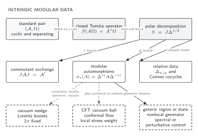
Tomita polar decomposition intrinsically produces commutant exchange, modular automorphisms, KMS structure, and the framework for comparing faithful states. Lorentz boosts for a vacuum wedge and conformal Killing flow for a CFT vacuum ball are conditional theorems; a generic region or state instead calls for spectral, kernel, or perturbative control. Schematic.

Read the lower arrows as extra deductions, not definitions. A correct calculation of $\Delta$ establishes modular flow. Identifying that flow with a boost, a conformal map, or an emergent translation is a separate claim with a separate hypothesis list.

What the chapter establishes

The first four pages build the operator-algebraic core. Modular Hamiltonians and their domains distinguish one-sided, standard, and relative generators. Tomita–Takesaki flow constructs $S$, $J$, and $\Delta$. Relative modular operators and Connes cocycles compare faithful states, while modular conjugation and commutants explain what $J$ exchanges and why it is not generically a spacetime reflection.

The next four pages move from structure to exact examples and observable consequences. The Bisognano–Wichmann theorem fixes vacuum-wedge flow and its $2\pi$ normalization. Conformal ball flow transports that result to a CFT causal diamond. Modular KMS correlators fix the analyticity strip and operator ordering, and modular spectral measures replace a misleading discrete “entanglement spectrum” by the appropriate spectral object.

The final four pages ask how much geometry can be inferred and how much explicit control remains without it. Half-sided modular inclusions generate positive translations under a one-sided compression theorem. Modular intersections combine compatible inclusions into larger symmetry relations. Nonlocal generators organize Gaussian, resolvent, and perturbative access with explicit errors. The convention atlas then translates signs, complements, additive constants, physical time, and absorbed $2\pi$ factors among the exact examples.

The division of labor matters. This chapter owns physical interpretation and controlled examples. A theorem-first treatment of general standard von Neumann algebras belongs to Tomita–Takesaki theory in mathematical QFT, while accelerated observers and curved horizons belong to the curved-spacetime modular treatment.

A convention you can carry through the chapter

The chapter fixes

$$K_{\rm std}=-\log\Delta, \qquad \sigma_s(A)=\Delta^{is}A\Delta^{-is} =e^{-isK_{\rm std}}Ae^{isK_{\rm std}}.$$

The parameter $s$ is dimensionless. Five consequences prevent most sign and interpretation errors.

1. The KMS strip follows the direction of flow. For analytic $A,B\in\mathcal A$, $F_{A,B}(z)=\omega(A\sigma_z(B))$ is analytic in the lower unit strip and obeys

   $$F_{A,B}(s-i)=\omega(\sigma_s(B)A).$$

   Replacing $\sigma_s$ by $\sigma_{-s}$ moves the strip to $0<\operatorname{Im}z<1$ and changes the boundary formula with it.

2. The wedge sign must be stated with the geometric action. For the right wedge, one convention used here is

   $$\Delta_W^{is}=U(\Lambda_W(-2\pi s)).$$

   Reversing the boost-rapidity convention or using $\Delta^{-is}$ reverses the sign. The magnitude $2\pi$ is fixed by the modular/KMS normalization.

3. Thermal time is a special identification. If $\rho_\beta=Z^{-1}e^{-\beta H}$ and $\tau_t(A)=e^{itH}Ae^{-itH}$, then

   $$\sigma_s(A)=\rho_\beta^{is}A\rho_\beta^{-is} =\tau_{-\beta s}(A).$$

   Modular time is not physical time for a generic subregion.

4. Constants and supports do different things. Adding $c\mathbf1$ to a one-sided $K_\rho$ leaves its adjoint action unchanged. Removing the kernel of $\rho$ changes the support algebra on which the logarithm exists.

5. Antiunitarity changes exponential bookkeeping. Although $J(-\log\Delta)J=\log\Delta$, the complex conjugation of $i$ compensates the generator sign, giving $J\Delta^{is}J=\Delta^{is}$ for real $s$. Moving $i$ through $J$ as though $J$ were unitary gives the wrong answer.

Whenever another source uses a different convention, translate the complete adjoint action and one KMS boundary equation. Comparing only the symbol $K$ is insufficient.

Representative modular flows and their boundaries

The table is the chapter’s common reference. “Exact” means exact for the stated algebra, state, representation, and hypotheses. It does not mean that the generator is bounded, local, or easy to compute.

Representative modular constructions and the strongest conclusion licensed in each domain

Construction	Modular object	Exact conclusion	Essential hypotheses	Failure test
Faithful finite matrix state	One-sided −log ρ; standard-form Δ acts by left ρ and right inverse ρ	Discrete ratio spectrum, exact adjoint flow, and direct finite KMS identities	Fixed algebra and representation; positive density matrix or explicit support reduction	Insert a zero eigenvalue or keep ρ fixed while changing the represented algebra
Vacuum Rindler wedge	Wedge modular operator; one-sided stress-tensor boost charge when that representative is available	Lorentz boosts preserving the wedge with fixed 2π normalization	Poincaré covariance, locality, positive energy, invariant vacuum, standard wedge algebra, and analytic field control	Use an excited state or a regulator that breaks the covariance and analytic hypotheses
CFT vacuum ball	Ball modular operator; a one-sided regulated or split representative is a local stress-tensor integral with quadratic radial weight	Conformal Killing flow preserving the causal diamond	Conformal covariance, conformal vacuum, round ball, and the wedge theorem	Add a relevant deformation, excite the state, or deform the sphere
Equilibrium full algebra	Gibbs logarithm in a regulator, or algebraic KMS modular data	Modular flow equals physical evolution after the chosen β rescaling	The state is KMS for the stated physical dynamics and the sign convention is fixed	Restrict to a generic subregion or compare with a different Hamiltonian
Half-sided modular inclusion	Two modular groups in a one-sided inclusion; a closed positive translation generator	Affine dilation–translation relations and positive translations	Common cyclic and separating vector for the stated algebras and the specified half-sided modular condition	Reverse the half side without changing conventions, or drop the inclusion condition
Generic QFT region and state	Unbounded log Δ and bounded unitary powers; often only spectral measures or controlled kernels are accessible	Exact algebra automorphism and intrinsic KMS structure; no general spacetime action	Cyclic and separating state for the stated algebra; domains for every unbounded refinement	Fit a local stress-tensor weight without a geometric theorem, or extrapolate a cutoff eigenvalue list as continuum spectrum

The geometric rows rest on distinct primary results. Bisognano and Wichmann identify the wedge modular objects from relativistic analyticity and locality Bisognano and Wichmann 1975, Theorem 2 and §§V–VI, pp. 997–1001. The ball flow follows by conformally mapping the wedge and checking both invariance and the KMS condition Casini, Huerta, and Myers 2011, §2.1, eqs. (2.11)–(2.20). For a negative half-sided inclusion, the completed theorem constructs a strongly continuous positive translation group and proves the affine scaling law from the one-sided modular hypothesis Araki and Zsidó 2005, Theorem 2.1 and eqs. (2.19)–(2.21). This is the domain-complete form of the result initiated by Wiesbrock 1993, pp. 83–92 and the 1997 erratum.

A guided route

If this is your first encounter with modular theory, begin with the finite Hilbert–Schmidt model on the first two pages. Work out $\Delta(E_{ij})=(p_i/p_j)E_{ij}$ before reading the continuum discussion. That calculation makes the complementary inverse, reciprocal spectrum, and unbounded logarithm concrete. Then read the wedge and KMS pages together: the wedge supplies geometry, while the KMS boundary equation checks its normalization.

If your goal is continuum entanglement or relative entropy, read the domain page, Tomita–Takesaki flow, and the relative modular page before using any formula of the form $-\log\rho_A$. Keep the algebra fixed when comparing states, write the support condition, and record the vector on which $\log\Delta_{\phi\mid\psi}$ is evaluated. A cocycle is an ordered, transported product; it is not generically the exponential of a difference of noncommuting logarithms.

If your goal is spacetime reconstruction, first master the wedge theorem and modular conjugation. Then read half-sided inclusions before intersections. The logical chain is

$$\text{standard algebras} \longrightarrow \text{half-sided or intersection relations} \longrightarrow \text{positive generators} \longrightarrow \text{geometric interpretation}.$$

An unlabeled collection of modular spectra skips the relations that do the reconstructive work.

If your goal is computation, pair the spectral-measure and nonlocal-generator pages. A finite cutoff always gives discrete eigenvalues, whereas a continuum statement may require convergence of resolvents, vector spectral measures, quadratic forms, or smeared correlators. Report the topology and the error actually controlled.

When a modular-flow claim is licensed

A modular claim can fail at four logically independent gates: the object may change, the generator may be used outside its domain, a geometric theorem may be missing, or a reconstruction theorem may be invoked without its inclusion relations. The decision map keeps those gates separate.

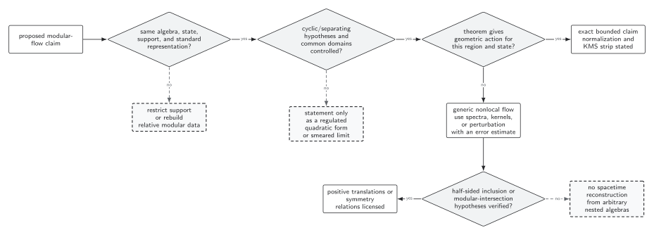
A bounded modular unitary can remain exact when an unbounded logarithm or commutator is uncontrolled. Exact geometric action additionally requires a theorem for the stated region and state. Positive translations or spacetime organization require verified half-sided-inclusion or modular-intersection hypotheses; arbitrary nesting or similar spectra do not suffice. Schematic.

Use four adversarial tests throughout the chapter.

• Change the support. Send one eigenvalue of a finite density matrix to zero. The adjoint flow may survive on the reduced support, while an inverse or full-space logarithm ceases to exist.
• Probe the domain. Choose a vector whose spectral measure makes $\int |\log\lambda|^2\,d\mu(\lambda)$ diverge. The unitary powers of $\Delta$ still act, but $K\xi$ does not exist.
• Break the geometric hypotheses. Excite the wedge vacuum, deform a CFT ball, or use a Lorentz-breaking cutoff. The algebraic modular flow remains meaningful, but the exact boost or conformal Killing formula is no longer licensed.
• Break the modular position. Reverse or perturb a half-sided inclusion so that its one-sided compression fails. Ordinary nesting remains, but the positive-translation conclusion does not follow.

The strongest defensible statement is the one that survives the relevant test. A regulated quadratic form, a smeared spectral measure, or a finite-time approximation can be valuable without being promoted to an exact local generator.

Check your preparation

1. A faithful two-level state has eigenvalues $p$ and $1-p$. What does the standard modular operator do to $E_{12}$, and why is this not a one-sided entanglement energy?

Answer

In the Hilbert–Schmidt standard representation,

$$\Delta(E_{12})=\frac{p}{1-p}E_{12}, \qquad K_{\rm std}(E_{12})=-\log\!\frac{p}{1-p}\,E_{12}.$$

The eigenvalue is a ratio, and the modular-generator eigenvalue is a difference of one-sided levels. A one-sided entanglement energy is either $-\log p$ or $-\log(1-p)$; only their difference appears here.

2. With $\sigma_s(A)=\Delta^{is}A\Delta^{-is}$, which KMS strip should you use?

Answer

Use the lower unit strip $-1<\operatorname{Im}z<0$ for $F_{A,B}(z)=\omega(A\sigma_z(B))$, with

$$F_{A,B}(s-i)=\omega(\sigma_s(B)A).$$

If you reverse modular time, the equivalent formulation uses the upper unit strip. The flow direction, imaginary shift, and operator ordering must be changed together.

3. Why does “the boost preserves the wedge” not determine modular flow?

Answer

Region preservation fixes neither the rapidity orientation nor the conversion between rapidity and dimensionless modular time. Relativistic analyticity, locality, the vacuum, and the spectrum condition identify the Tomita boundary relation and fix the $2\pi$ normalization. Without that input, a wedge-preserving one-parameter group is only a candidate symmetry.

4. What survives when a ball in a CFT is smoothly deformed away from a sphere?

Answer

The algebra–state pair still has modular flow when the state is cyclic and separating. What is lost is the exact conformal equivalence to a wedge and hence the simple local quadratic stress-tensor kernel. A controlled shape expansion may supply null or nonlocal corrections with a stated remainder; substituting a position-dependent radius into the sphere formula is not an exact derivation.

5. Does every nested pair of local algebras generate a translation?

Answer

No. The theorem uses a common cyclic and separating vector and a modular group that compresses the smaller algebra for one sign of modular time. Under the completed negative half-sided theorem, strong continuity and positivity of the resulting translation group are conclusions. Stronger reconstruction statements require additional standard relative-position and compatibility hypotheses. Ordinary isotony alone gives none of the affine commutation relations.

References

• Araki, Huzihiro. “Relative Entropy of States of von Neumann Algebras.” Publications of the Research Institute for Mathematical Sciences 11 (1976): 809–833. DOI and open article.
• Araki, Huzihiro, and László Zsidó. “Extension of the Structure Theorem of Borchers and Its Application to Half-Sided Modular Inclusions.” Reviews in Mathematical Physics 17 (2005): 491–543. DOI. Open article.
• Bisognano, Joseph J., and Eyvind H. Wichmann. “On the Duality Condition for a Hermitian Scalar Field.” Journal of Mathematical Physics 16 (1975): 985–1007. DOI. Open PDF.
• Casini, Horacio, Marina Huerta, and Robert C. Myers. “Towards a Derivation of Holographic Entanglement Entropy.” Journal of High Energy Physics 05 (2011): 036. DOI. Open PDF.
• Takesaki, Masamichi. Tomita’s Theory of Modular Hilbert Algebras and Its Applications. Lecture Notes in Mathematics 128. Berlin: Springer, 1970. DOI.
• Wiesbrock, Hans-Werner. “Half-Sided Modular Inclusions of von-Neumann-Algebras.” Communications in Mathematical Physics 157 (1993): 83–92; erratum 184 (1997): 683–685. DOI.
• Witten, Edward. “Notes on Some Entanglement Properties of Quantum Field Theory.” Reviews of Modern Physics 90 (2018): 045003. DOI. Open PDF.