Modular Response and Quantum Information Geometry

A modular-response coefficient is a derivative, so its meaning begins with a deceptively simple question: what is varied, and what is held fixed? Varying a state on one algebra, moving the region that defines the algebra, choosing a quantum information metric, and transporting modular eigenspaces are different operations. They can share formulas without defining the same observable.

This chapter develops those operations from one common starting point: relative entropy with a fixed reference. Density matrices provide the clearest regulated formulas. In continuum QFT, local algebras are generally type III, so relative modular operators and algebraic relative entropy replace reduced density matrices and separately divergent entropies. The finite-dimensional equations below are therefore both a derivation and a checklist for taking a controlled QFT limit.

Helpful background. Modular Hamiltonian definitions fix domains and additive conventions, relative entropy in QFT supplies the finite comparison, and out-of-time-order correlators clarify why analytic growth is not by itself a diagnosis of physical chaos.

Enter a differentiable family

Let $\rho_\lambda$ be a normalized $C^3$ family of faithful states on one fixed regulated algebra, with

$$\rho_0=\sigma, \qquad X\equiv \dot\rho_0, \qquad \operatorname{Tr}X=0, \qquad K_\sigma=-\log\sigma.$$

The exact fixed-reference identity is

$$D(\rho_\lambda\Vert\sigma) =\Delta\langle K_\sigma\rangle-\Delta S,$$

where each $\Delta$ subtracts its value in $\sigma$. Because relative entropy has a minimum at $\rho_\lambda=\sigma$, its linear term vanishes. Differentiating the exact identity at $\lambda=0$ gives the entanglement first law

$$\delta S=\delta\langle K_\sigma\rangle.$$

The reference modular Hamiltonian is held fixed. The first law does not say that the entropy equals modular energy at finite $\lambda$, nor does it license differentiating a first-order equality a second time. Instead, one differentiates the exact relative-entropy identity again. For a faithful regulated state,

$$D(\rho_\lambda\Vert\sigma) =\frac{\lambda^2}{2}\, g_{\mathrm{KM},\sigma}(X,X) +O(\lambda^3),$$

with the Bogoliubov–Kubo–Mori quadratic form

$$g_{\mathrm{KM},\sigma}(X,X) =\operatorname{Tr}\!\left[X\,D\log(\sigma)[X]\right], \qquad D\log(\sigma)[X] =\int_0^\infty dt\, (\sigma+t)^{-1}X(\sigma+t)^{-1}.$$

This form is nonnegative and vanishes only for a zero tangent on the faithful support. The derivation and its QFT interpretation are given in Blanco, Casini, Hung, and Myers 2013, §2; the algebraic continuum object originates with Araki 1976, pp. 809–815.

A two-level commuting check makes the boundary behavior concrete. For $\sigma=\operatorname{diag}(p,1-p)$ and $X=x\operatorname{diag}(1,-1)$,

$$g_{\mathrm{KM},\sigma}(X,X) =x^2\!\left(\frac{1}{p}+\frac{1}{1-p}\right) =\frac{x^2}{p(1-p)}.$$

It is the ordinary classical Fisher metric and diverges as the reference loses support. Noncommuting tangents retain this support sensitivity but split into inequivalent quantum metrics.

The diagram separates the exact comparison identity from the distinct derivatives built from it. In particular, the positive Hessian is not obtained by extending the first law beyond first order.

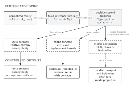
Fix the reference, algebra or algebra identification, support, and tangent before differentiating. The first law and positive relative-entropy Hessian are separate derivatives of the exact fixed-reference identity; shape response and modular transport require additional pullback or projection data. The diagram is schematic and not to scale.

The chapter has three connected reading paths. For state response, begin with the entanglement first law and quadratic correction, then construct a finite state susceptibility. For moving regions, use the separate shape-deformation framework before evaluating stress-tensor response kernels; the leading deformed-half-space formula and its null-horizon terms are derived in Faulkner, Leigh, Parrikar, and Wang 2016, §§2–3.

For information geometry, start with symmetric-logarithmic-derivative quantum Fisher information, compare Bures, Kubo–Mori, and other monotone metrics, and then isolate universal information in fidelity susceptibility under relevant deformations. The final sequence develops modular Berry holonomy, conditional modular analyticity bounds, noncommutative exponential families, and a practical contact-term, domain, and error budget.

Independent validity gates

A finite positive number is not yet a physical susceptibility. Five logically independent checks stand between a formal derivative and an interpretable result:

1. The state family is normalized, and either the algebra is fixed or moving algebras are identified by an explicit pullback.
2. The tangent lies in a common support and operator domain, with the required smearing or energy restriction.
3. Contact, boundary, improvement, and regulator terms are kept in the same scheme on both sides of every comparison.
4. The metric, operator ordering, analytic strip, and experimental or computational proxy are named explicitly.
5. Perturbative truncation, finite-size, statistical, and numerical errors are bounded separately.

Passing one gate does not repair another. Positivity cannot remove a contact ambiguity; analyticity cannot choose a metric; a small numerical residual cannot establish that a continuum operator exists.

Normalization or algebra identification, tangent-domain control, consistently treated contact and regulator terms, interpretation conventions, and error control are independent. An unresolved error licenses only an estimate with that limitation; it does not establish a controlled regulator limit. The decision map is schematic and not to scale.

A reproducible calculation should therefore report the regulated family, reference and support; the tangent or shape-identification map; the kernel and ordering; all contact and boundary terms; the metric normalization; and an error budget. For a metric or susceptibility, establish a finite positive regulated quadratic form, test its stability under smearing and regulator changes, and only then attach an operational interpretation. Holonomy instead begins with a smooth isolated projector and controlled unitary transport; an analytic growth claim begins with a named correlator, proven strip and boundary bound, and controlled errors.

Comparison of information geometries

For noncommuting families, “the quantum Fisher metric” is not unique. This chapter uses the symmetric logarithmic derivative $L$ defined by $X=(\sigma L+L\sigma)/2$ and

$$F_Q=\operatorname{Tr}(\sigma L^2), \qquad ds_B^2=\frac14 F_Q\,d\lambda^2.$$

The chapter writes root fidelity as $f=\operatorname{Tr}\sqrt{\sqrt\rho\,\sigma\sqrt\rho}$ and squared fidelity as $F=f^2$, with $D_B^2=2(1-f)$. Readers should translate factors of two or four before comparing sources that call either $f$ or $F$ “fidelity.” The estimation normalization follows Braunstein and Caves 1994, pp. 3440–3442; the classification and ordering of monotone metrics follow Petz 1996, pp. 87–90. Every row below assumes a normalized tangent and a declared common support.

Information metrics and modular responses for controlled quantum-state families.

Construction	Family and tangent	Normalization or kernel	Positivity and monotonicity	Continuum control	Operational or computational proxy
SLD quantum Fisher information	Faithful density operators, or a fixed-support extension, with tangent equal to one-half of ρL + Lρ	Fisher information is Tr ρL²; the corresponding Bures line element is one quarter of this value	Positive and contractive under quantum channels; gives the smallest normalized monotone metric	Sharp local parameter directions can diverge; specify smearing, support, and energy control	Maximum classical Fisher information over measurements and the quantum Cramér–Rao bound
Bures metric	State family compared through Uhlmann fidelity, including a controlled fixed-support boundary limit	One quarter of SLD Fisher information when Bures distance is defined by 2(1 − root fidelity)	Positive and channel contractive; four times the geometric Bures metric is the minimal Petz-normalized monotone metric	Continuum fidelity requires one comparison algebra and a regulator-safe limit	Purification distance, optimal purification overlap (or pure-state overlap), and locally optimal estimation
Bogoliubov–Kubo–Mori metric	Faithful noncommuting family, naturally described in exponential coordinates	Hessian of relative entropy or log partition function with the logarithmic-mean kernel	Positive and channel contractive; equals the classical Fisher metric on commuting directions but generally exceeds SLD with matched normalization	Relative quantities can cancel state-independent UV terms, but tangent-domain and contact checks remain	Static susceptibility, imaginary-time connected correlators, and relative-entropy response
Fidelity susceptibility	Ground-state, thermal, or reduced-state family under a named parameter deformation	Quadratic fidelity loss; its factor relative to Fisher information depends on rooted-versus-squared fidelity convention	Nonnegative, while extensivity, singularity, and critical scaling are model and direction dependent	Often contains volume and cutoff terms; universal parts require subtraction or finite-size scaling	Overlap derivatives, spectral sums, and integrated deformation correlators
Relative-entropy modular response	Fixed algebra and reference state with a differentiable normalized tangent	Second variation of relative entropy; the Kubo–Mori metric in the faithful regulated setting	Positive and monotone under restriction or quantum channels	Often the most robust continuum comparison after matched UV terms cancel	Modular-flow kernels, stress-tensor response, and regulated correlator differences

What the chapter establishes

The chapter establishes exact differential identities for faithful regulated families and specifies the additional hypotheses needed in continuum QFT. It does not identify one information metric as universally measurable, equate every susceptibility peak with a phase transition, or infer physical chaos from modular KMS analyticity alone. Modular Berry transport is defined only after the zero-mode sector and degeneracies are controlled; its geometric interpretation is model dependent, as the symmetric two-dimensional CFT construction makes explicit in Czech, Lamprou, McCandlish, and Sully 2018, pp. 2–4.

The preceding chapter on modular operators and geometric flow supplies the modular generator and domain theory used here. The next chapter on information across scales and renormalization applies these response tools to theory-space directions and RG flow, where scheme dependence and scale matching become central.

References

• Araki, Huzihiro. “Relative Entropy of States of von Neumann Algebras.” Publications of the Research Institute for Mathematical Sciences 11 (1976): 809–833. DOI.
• Blanco, David D., Horacio Casini, Ling-Yan Hung, and Robert C. Myers. “Relative Entropy and Holography.” Journal of High Energy Physics 2013, no. 8 (2013): 060. DOI; arXiv.
• Braunstein, Samuel L., and Carlton M. Caves. “Statistical Distance and the Geometry of Quantum States.” Physical Review Letters 72 (1994): 3439–3443. DOI.
• Czech, Bartłomiej, Lampros Lamprou, Samuel McCandlish, and James Sully. “Modular Berry Connection for Entangled Subregions in AdS/CFT.” Physical Review Letters 120 (2018): 091601. DOI; arXiv.
• Faulkner, Thomas, Robert G. Leigh, Onkar Parrikar, and Huajia Wang. “Modular Hamiltonians for Deformed Half-Spaces and the Averaged Null Energy Condition.” Journal of High Energy Physics 2016, no. 9 (2016): 038. DOI; arXiv.
• Petz, Dénes. “Monotone Metrics on Matrix Spaces.” Linear Algebra and its Applications 244 (1996): 81–96. DOI.