Operator Entanglement and Channel–State Maps

Operator entanglement asks how far an evolution operator or channel is from factorizing across a spatial cut. In finite dimension, vectorization turns the map into a normalized state on doubled input and output systems. In a field theory, the equal-weight maximally entangled vector is not normalizable and local continuum algebras need not be type-I tensor factors. A meaningful dynamical diagnostic therefore states the regulator, doubled partition, reference energy, normalization, and order of cutoff and reference-state limits.

Required background. Tensor products and index structure supplies the doubled-space partition, and channel–state methods in infinite dimensions supplies the reconstruction domain and type-III cautions.

Helpful background. Entanglement growth supplies the physical-state comparison, while energy-constrained channel distances supplies a class-wide topology for bosonic channels.

Vectorizing a finite-dimensional evolution

Let the physical system factor as $\mathcal H_A\otimes\mathcal H_B$, with dimensions $d_A$ and $d_B$. Introduce copies $A'$ and $B'$ and the normalized reference

$$|\Omega\rangle =\frac{1}{\sqrt{d_Ad_B}} \sum_{i=1}^{d_A}\sum_{j=1}^{d_B} |i,j\rangle_{AB}|i,j\rangle_{A'B'}.$$

For a unitary $U(t)$, define

$$|U(t)\rangle\!\rangle =\bigl(U_{AB}(t)\otimes\mathbf1_{A'B'}\bigr)|\Omega\rangle.$$

The spatial operator entanglement is the entropy across

$$(AA'):(BB'),$$

not across output versus input. The latter cut has a different meaning and, for a unitary acting on half of a maximally entangled reference, is fixed by construction. Indeed, tracing out the reference leaves

$$\rho_{AB}=U\frac{\mathbf 1_{AB}}{d_A d_B}U^\dagger =\frac{\mathbf 1_{AB}}{d_A d_B}, \qquad S_{AB:A'B'}=\log(d_A d_B).$$

This value is therefore the normalization of the doubled reference, not a measure of how strongly $U$ couples the spatial factors $A$ and $B$. A basis is needed to define vectorization, but local basis changes act as local unitaries on the doubled spatial factors and do not change the Schmidt spectrum.

The doubled-space bookkeeping is easiest to see geometrically. In the figure, follow the vertical dashed cut: each physical factor stays with its own reference copy before the spatial partition is made. Rotating the cut by ninety degrees instead separates the channel output from its reference input and answers a different question.

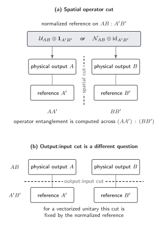
Doubled-space bookkeeping. The channel acts only on the physical factors $AB$. Spatial operator entanglement uses the vertical cut $(AA'):(BB')$; the horizontal output:input cut $AB:A'B'$ defines a different quantity and, for a normalized vectorized unitary, has entropy $\log(d_A d_B)$. The diagram is schematic and not to scale.

If $U=U_A\otimes U_B$, then

$$|U\rangle\!\rangle =|U_A\rangle\!\rangle_{AA'} \otimes|U_B\rangle\!\rangle_{BB'},$$

so $S_{\rm op}(U)=0$. Conversely, for a bipartite unitary in finite dimension, zero operator entanglement across this cut identifies a product operator up to the normalization convention. Zanardi 2001, Eqs. (2)–(9) develops this operator-state correspondence and distinguishes operator entanglement from entangling power.

The diagnostic depends on the entropy functional. The von Neumann operator entropy is

$$S_{\rm op}(U)=-\operatorname{tr}\rho_{AA'}^{(U)} \log\rho_{AA'}^{(U)},$$

whereas the linear operator entropy is $1-\operatorname{tr}[(\rho_{AA'}^{(U)})^2]$. Quote which one is used; their numerical ranges and scaling differ.

Identity and SWAP are decisive controls

For equal local dimension $d$, the identity channel state factorizes and has $S_{\rm op}(\mathbf1)=0$. The SWAP operator gives

$$|{\rm SWAP}\rangle\!\rangle =\frac1d\sum_{i,j=1}^{d} |j,i\rangle_{AA'}|i,j\rangle_{BB'}.$$

This is already a Schmidt decomposition with $d^2$ equal probabilities $1/d^2$. Therefore

$$S_{\rm op}({\rm SWAP})=2\log d, \qquad E_{\rm op}^{\rm linear}({\rm SWAP})=1-\frac1{d^2}.$$

For $d=3$, the von Neumann value is $2\log3\approx2.197225$. Yet SWAP maps every unassisted product state $|a\rangle|b\rangle$ to the product $|b\rangle|a\rangle$. Its ordinary unassisted entangling power is zero. This exact contrast prevents a large operator entropy from being misreported as entanglement generated from every physical input.

Operator entanglement also does not, by itself, prove scrambling. A large value already occurs in integrable dynamics: Prosen and Pižorn 2007, § III and Figs. 1–2 exhibit operator-space entanglement growth in the transverse Ising chain and explain its computational significance. Comparisons between dynamical classes must hold the cut and Rényi index fixed and add a scaling law plus an independent operator-growth or recovery diagnostic.

Channels and channel-state mixedness

For a channel $\mathcal N$ rather than a unitary, apply $\mathcal N$ to the physical half of $|\Omega\rangle\langle\Omega|$. The resulting Choi state is generally mixed, but it is pure exactly for Choi rank one—a single-Kraus isometry, which in equal input and output dimensions is a unitary channel. When the Choi state is mixed, its subsystem entropy is not an entanglement measure. Possible diagnostics include:

• mutual information across $(AA'):(BB')$ for total correlation;
• logarithmic negativity for one mixed-state entanglement test;
• operator-space Rényi entropy of a chosen superoperator representation;
• recovery or decoupling performance for an operational task.

These quantities can order channels differently. State the trace normalization, input reference, bipartition, and whether the environment or measurement record is retained. A channel-state entropy averaged over records is not the average entropy of conditioned channel states.

A finite-energy bosonic reference

There is no normalized equal-weight vector $\sum_{n=0}^\infty|n,n\rangle$ for an oscillator. Replace it by the two-mode squeezed vacuum

$$|\Omega_r\rangle =\sqrt{1-\lambda^2} \sum_{n=0}^{\infty}\lambda^n|n\rangle_{\rm out}|n\rangle_{\rm in}, \qquad \lambda=\tanh r.$$

The Schmidt probabilities are

$$p_n=(1-\lambda^2)\lambda^{2n}.$$

Each half has mean occupation and entropy

$$N=\frac{\lambda^2}{1-\lambda^2}=\sinh^2r, \qquad g(N)=(N+1)\log(N+1)-N\log N.$$

$N$ is dimensionless occupation, not energy. For $H=\omega a^\dagger a$, the excitation energy is $\omega N$ per half and $2\omega N$ for the pair, excluding zero-point terms. For several modes with squeezing profile $r_k$, the resource per half is

$$E_{\rm ref}-E_0=\sum_k\omega_k\sinh^2r_k.$$

Apply the regulated evolution to the output half of each chosen local or wavepacket mode, assemble the doubled covariance, and calculate the entanglement across a spatially defined $(AA'):(BB')$ cut. A momentum-mode cut is a different observable. The reference mode functions and spatial regulator are therefore part of the definition.

Infinite-dimensional Gaussian Choi–Jamiolkowski forms and their operator domains are developed by Holevo 2011, §§ 2–5. For every finite $r>0$, all probabilities $p_n$ are nonzero, so the squeezed reference has full Fock-basis support. Reconstructing high-excitation matrix elements is nevertheless poorly conditioned: it requires division by Schmidt weights that decay geometrically with $n$.

A finite-energy Gaussian channel benchmark

Consider two equal-frequency physical oscillators $A,B$ and references $A',B'$. Prepare two independent squeezed pairs,

$$|\Psi_0\rangle =|\Omega_r\rangle_{AA'}\otimes|\Omega_r\rangle_{BB'},$$

and apply a beam-splitter evolution only to the physical oscillators:

$$\begin{aligned} q_A^{\rm out}&=\cos\theta\,q_A+\sin\theta\,q_B, \\ q_B^{\rm out}&=-\sin\theta\,q_A+\cos\theta\,q_B,\\ p_A^{\rm out}&=\cos\theta\,p_A+\sin\theta\,p_B, \\ p_B^{\rm out}&=-\sin\theta\,p_A+\cos\theta\,p_B. \end{aligned}$$

This is an energy-preserving Gaussian unitary channel. With one-mode vacuum covariance $\mathbf1_2/2$, define

$$\begin{aligned} c&=\cosh 2r,\\ s&=\sinh 2r,\\ Z&=\operatorname{diag}(1,-1). \end{aligned}$$

Here $\mathbf1_2$ is the identity on one mode’s two quadratures.

After the channel, the reduced covariance on the spatial factor $(A_{\rm out},A')$ is

$$\Gamma_{AA'}^{\rm out} =\frac12 \begin{pmatrix} c\mathbf1_2 & s\cos\theta\,Z\\ s\cos\theta\,Z & c\mathbf1_2 \end{pmatrix}.$$

Its two symplectic eigenvalues are equal:

$$\begin{aligned} \nu_1=\nu_2 &=\frac12\sqrt{c^2-s^2\cos^2\theta}\\ &=\frac12\sqrt{1+\sin^2\theta\,\sinh^2 2r}. \end{aligned}$$

Because the four-mode channel state is pure, the spatial operator entanglement is

$$S_{\rm op}(r,\theta) =2g\!\left(\nu_1-\frac12\right).$$

The controls are decisive. At $\theta=0$, the channel is spatially factorized and $S_{\rm op}=0$. At $\theta=\pi/2$, it swaps the two physical modes and

$$S_{\rm op}=2g(\sinh^2r),$$

the finite-energy analogue of the finite-dimensional SWAP result. For $r=0.5$, $\theta=\pi/4$, and unit oscillator frequency,

$$\begin{aligned} N&=\sinh^2(0.5)\approx0.271540,\\ E_{\rm ref}-E_0&=2N\approx0.543081,\\ \nu_1=\nu_2&\approx0.650106,\\ S_{\rm op}&\approx0.891018\ {\rm nats}. \end{aligned}$$

Here $E_{\rm ref}$ counts the two reference modes $A',B'$; the full doubled probe carries twice that excitation. This is a reproducible finite-energy channel-state calculation, not an infinite-squeezing extrapolation.

Cutoff convergence can be checked independently. If each squeezed pair is truncated at $n\leq N_c$, its omitted probability is $\epsilon=\lambda^{2(N_c+1)}$, and the probability omitted from either of the two independent pairs is

$$\epsilon_{\rm two}=1-(1-\epsilon)^2.$$

For $r=0.5$ and $N_c=8$, $\epsilon_{\rm two}\approx1.85\times10^{-6}$. Increasing $N_c$ at fixed $r$ controls the representation error; changing $r$ changes the physical reference and therefore legitimately changes $S_{\rm op}$.

Two limits that must not be merged

At fixed squeezing $r$ and a Fock cutoff $0\leq n\leq N_c$, the omitted reference probability is

$$\epsilon_{N_c}=\sum_{n=N_c+1}^{\infty}p_n =\lambda^{2(N_c+1)}.$$

First increase $N_c$ at fixed $r$, reference mode, and physical energy. Only after the cutoff tail and output observables converge should the reference energy or squeezing profile be varied. Increasing $r$ and $N_c$ together can conceal a changing physical probe behind an apparently stable matrix size.

There is no normalized $r\to\infty$ limit: $N$ and the reference energy diverge. Stability at one large $r$ is not a continuum invariant. Nor does stability for one squeezed probe imply uniform accuracy for every input with energy below $E$. A class-wide channel statement requires a metric such as

$$\|\Phi-\Psi\|_{\diamond,E,H} =\sup_{\operatorname{tr}(H\rho_A)\leq E} \left\|[(\Phi-\Psi)\otimes\operatorname{id}_R](\rho_{AR})\right\|_1,$$

with the Hamiltonian and admissible ancilla declared. Shirokov 2018, § 4 establishes the role of this energy-constrained topology.

For a continuum local QFT algebra, an additional issue remains: type-III locality need not supply a canonical density matrix or tensor-factor trace. A split inclusion, selected modes, or lattice regulator can define the doubled diagnostic, but the result belongs to that construction. The dedicated infinite-dimensional channel–state page develops this boundary in detail.

Reproducible operator-entanglement protocol

1. State the finite regulator or selected mode algebra and its Hamiltonian.
2. Draw or write the doubled partition explicitly.
3. Fix the vectorization normalization and entropy functional.
4. Run identity, product-unitary, and SWAP controls.
5. At fixed reference energy, converge Fock or local-Hilbert-space cutoffs.
6. Vary the reference energy and squeezing profile only after cutoff convergence.
7. Compare operator entropy with physical-state entanglement and an independent information task.

The chapter orientation map places this as a direct channel diagnostic rather than a state-entropy substitute. Its failure controls make estimator and reference changes explicit, and the diagnostic comparison records the required energy and cutoff window.

Common pitfalls

Partitioning output from input. Operator entanglement across a spatial cut uses $(AA'):(BB')$. A different doubled cut answers a different question.

Calling $\sinh^2r$ an energy. It is the mean occupation. Multiply by the declared mode frequency and include all modes.

Taking infinite squeezing. No normalized maximally entangled oscillator state appears in that limit. Keep an energy domain and report reference dependence.

Exercises

Derive the Schmidt spectrum and operator entropies of SWAP on $\mathbb C^d\otimes\mathbb C^d$. Why can its ordinary entangling power still vanish?

Solution

The vectorized state has $d^2$ orthonormal Schmidt pairs with amplitude $1/d$, so every probability is $1/d^2$. Hence

$$S_{\rm op}=-d^2\frac1{d^2}\log\frac1{d^2}=2\log d,$$

and $1-\sum p^2=1-1/d^2$. But ${\rm SWAP}|a\rangle|b\rangle=|b\rangle|a\rangle$, which remains a product for every product input. Operator nonfactorizability and state entangling power are different resources.

Starting from $p_n=(1-\lambda^2)\lambda^{2n}$, derive $N$, the cutoff tail, and the marginal entropy.

Solution

The geometric-series identity gives

$$N=(1-\lambda^2)\sum_{n=0}^{\infty}n\lambda^{2n} =\frac{\lambda^2}{1-\lambda^2}.$$

The tail is

$$(1-\lambda^2)\sum_{n=N_c+1}^{\infty}\lambda^{2n} =\lambda^{2(N_c+1)}.$$

Substituting the geometric probabilities into $-\sum p_n\log p_n$ and using the expression for $N$ yields $g(N)=(N+1)\log(N+1)-N\log N$.

Take $\lambda=1/2$, oscillator frequency $\omega=3$, and cutoff $N_c=4$. Find the mean occupation, excitation energy per half, and omitted probability.

Solution

The occupation is

$$N=\frac{1/4}{3/4}=\frac13.$$

The excitation energy per half is $\omega N=1$. The omitted probability is

$$\epsilon_4=\left(\frac12\right)^{10} =\frac1{1024}\approx9.7656\times10^{-4}.$$

Increasing $\lambda$ would change both the energy and this tail, so it is not a cutoff-only refinement.

References

• Holevo, Alexander S. “The Choi–Jamiolkowski Forms of Quantum Gaussian Channels.” Journal of Mathematical Physics 52 (2011): 042202. DOI.
• Prosen, Tomaž, and Iztok Pižorn. “Operator Space Entanglement Entropy in a Transverse Ising Chain.” Physical Review A 76 (2007): 032316. DOI.
• Shirokov, Maksim E. “On the Energy-Constrained Diamond Norm and Its Application in Quantum Information Theory.” Problems of Information Transmission 54 (2018): 20–33. DOI.
• Zanardi, Paolo. “Entanglement of Quantum Evolutions.” Physical Review A 63 (2001): 040304(R). DOI.