Information Across Scales and Renormalization

Information measures can reveal how distinguishability and long-range structure change from ultraviolet to infrared scales, but “scale dependence” is not yet an RG statement. Enlarging a region, removing a cutoff, changing a coupling, integrating out modes, and moving the renormalization scale are different operations. This chapter develops the entropic $c$ and $F$ functions and the four-dimensional $a$ inequality, then separates those theorems from finite crossovers, subtraction prescriptions, state channels, scale-space factorizations, and local metrics on families of theories.

Helpful background. Universal terms and geometry identifies the finite and logarithmic data used at conformal fixed points. Data processing supplies the information inequality behind genuine coarse-graining channels. UV and IR fixed points, flow constraints, and anomaly coefficients provide the RG and CFT endpoints.

Separate the scale roles before comparing

Five kinds of scale recur throughout the chapter:

• $\epsilon$ is a UV regulator length. A continuum limit sends $\epsilon/R\to0$ while the intended physical ratios remain fixed.
• $R$ describes the size of the chosen region. A second length $L$ can be a box size or the separation between disjoint regions; it is absent in a one-interval problem unless a finite box is introduced.
• $\xi$ is a correlation length of a state. It may be infinite at a critical point or may not exist as a single useful scale.
• A relevant scaling field $g_R(\mu)$ with linearized eigenvalue $y=d-\Delta>0$ defines a crossover length $\ell_g\propto |g_R|^{-1/y}$. The proportionality factor and the relation to $\xi$ depend on normalization and on the branch of the flow.
• $\mu^{-1}$ is the length associated with the renormalization convention. Physical answers can contain $\mu R$ while satisfying the appropriate RG equation.

These are distinct bookkeeping roles, not automatically independent variables. In a free massive vacuum, for example, $\xi$ and the deformation length are proportional to $m^{-1}$. Conversely, a flow to another CFT has a crossover scale but no finite IR correlation length. The dimensionless controls are therefore recorded before a calculation begins: typical examples are $R/\epsilon$, $L/R$, $R/\xi$, $R/\ell_g$, and $\mu R$.

The diagram summarizes the next decision. After fixing the comparison path, one must still decide whether the desired result is an endpoint theorem, a finite crossover, an operational channel statement, or a local response metric.

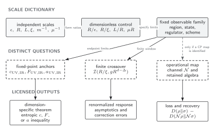
Scale and claim dictionary. Some scale roles can coincide or be absent; the calculation must record that fact rather than counting them as independent. The four lower branches answer different questions and require different evidence. Schematic and not to scale.

A safe numerical path makes this distinction operational. At each target value of $mR$, for instance, refine $R/\epsilon$ while holding $L/R$ fixed. Holding $m\epsilon$ fixed instead causes $mR=(m\epsilon)(R/\epsilon)$ to drift; a decreasing curve along that path can be a real massive crossover but is not evidence of cutoff convergence. Separating cutoff, region, correlation, and RG scales executes both paths on the same free-field regulator.

Four questions with different answers

The shortest route through the chapter depends on the claim one wants to make.

1. A dimension-specific theorem. Two-dimensional entropic monotones derives $c_E(R)=3R S'(R)$ from Lorentz symmetry and strong subadditivity. Three-dimensional F monotonicity develops $\mathcal F(R)=(R\partial_R-1)S(R)$ for vacuum disks. Four-dimensional a-type flow constraints distinguishes the endpoint inequality $a_{\rm UV}\ge a_{\rm IR}$ from particular dilaton and entropic proofs.
2. A finite crossover. Relevant deformations and crossovers fixes the scaling field and correction variables; renormalized entropy schemes compares differential, counterterm, and split mutual-information prescriptions on common data.
3. An operational loss of information. Relative entropy and irreversibility first constructs a common algebra or regulated embedding. Coarse-graining channels and recoverability then identifies an actual state map, its retained system, and the task against which recovery is judged.
4. A basis- or family-dependent diagnostic. Scale-space caveats compares Fourier and wavelet factorizations without calling basis dependence universal. Information geometry on theory space distinguishes normalized-state metrics from partition-function Hessians and removes unphysical coordinate redundancies only after boundaries and contact prescriptions are fixed.

The fixed-point theorem sources make the dimensional separation precise. The interval argument is given by Casini and Huerta 2007, pp. 7032–7035. The disk construction and $S''(R)\le0$ appear in Casini and Huerta 2012, § 4, Eqs. (16)–(24). Four-dimensional irreversibility follows from the positive dilaton-scattering sum rule of Komargodski and Schwimmer 2011, § 4, Eqs. (4.6)–(4.8), or from the null-cone entropic construction of Casini, Testé, and Torroba 2017, pp. 261602-2–261602-4. These results do not state that one formula is monotone in every dimension.

What a monotonicity claim must specify

A complete claim identifies all of the following:

1. the spacetime dimension and the hypotheses of the theorem being invoked;
2. the state and the declared family of regions as $R$ varies;
3. the regulator or algebraic construction that makes every comparison meaningful;
4. the subtraction, contact-term, or embedding prescription and the ambiguities it permits;
5. the direction in which the scale parameter runs;
6. the dimensionless ratios held fixed during refinement; and
7. the endpoint quantities or finite-window residuals that were actually checked.

The phrase “same region” is too strong: an entropic flow deliberately changes $R$. What must remain fixed is the region family and its prescription—for example, centered intervals in one vacuum or round disks on one time slice—together with the cutoff-refinement and subtraction rules. A half-site boundary shift, a changing shape, or a different finite counterterm can otherwise imitate flow.

Comparison table

The table is the semantic counterpart of the diagrams. It separates theorem-level conclusions from controlled but prescription-dependent diagnostics.

Information diagnostics compared by system, definition, hypotheses, finite-flow evidence, operational consequence, and characteristic failure.

Diagnostic	System	Definition or prescription	Hypotheses and endpoint anchor	Finite-flow evidence	Operational consequence	Adversarial failure
Entropic c-function	Vacuum interval in 1+1 dimensions	cE(R) = 3R S′(R)	Unitary Lorentz-invariant QFT and strong subadditivity; equals the CFT central charge at an endpoint	Correlated derivative fit with cutoff and box refinement	No recovery map is required for the theorem	A thermal state adds β and gives an increasing exact control curve
Renormalized F-function	Vacuum disk in 2+1 dimensions	𝓕(R) = (R∂R − 1)S(R)	Relativistic vacuum flow; equals the sphere free energy at a CFT	The differential operator itself removes the area term; fit-window and radial-cutoff stability remain to be checked	No recovery map is required for the entropic inequality	Raw disk entropy, a narrow fit window, or an untracked boundary contribution gives a false plateau
Four-dimensional a constraint	Smooth spheres or null-cone regions in 3+1 dimensions	Euler-anomaly endpoint difference; at a CFT the spherical logarithm is −4a log(R/ε)	Unitary relativistic flow between bulk CFTs; aUV ≥ aIR	Endpoint anomaly match or a controlled dilaton or null-cone calculation	No canonical finite a(R) and no generic recovery map follow	A finite counterterm, boundary anomaly, or non-CFT endpoint cannot be relabeled as bulk a
Renormalized entropy prescription	One scalable region family in a declared dimension	Dimension-dependent differential polynomial, fixed local counterterms, or symmetrically split mutual information	Surface geometry, framing, and subtraction convention fixed globally; fixed-point normalization checked	Agreement of universal endpoints and quantified prescription differences through the crossover	None by itself	Changing the split, fit, or counterterm between radii manufactures running
Relevant-deformation crossover	A fixed state and region family near an RG fixed point	Normalized scaling field gRRy, equivalently R/ℓg, plus irrelevant corrections	The scaling field, branch, nonuniversal metric factor, regulator path, and fit window declared	Data collapse, endpoint asymptotics, exponent stability, and correction-to-scaling residuals	A controlled crossover, not a theorem merely from collapse	Bare-coupling fits or coarse lattices can shift the apparent exponent
Relative-entropy diagnostic	Two normal states on one regional algebra, or one common type-I regulator	Araki relative entropy; on a regulated factor, D = Δ⟨K⟩ − ΔS	Support condition and reference state fixed; a cross-theory comparison needs an explicit embedding	Region-size dependence, conditioning, continuum refinement, and endpoint asymptotics	Recovery follows only after a restriction or channel is specified and its loss is controlled	Changing only one state’s embedding changes the answer
Coarse-graining channel	Retained regulated subsystem, or a continuum subalgebra	CPTP state map in type I; predual of a normal unital completely positive algebra map in the continuum	Input, output, reference state, side information, and operational task fixed	Finite distinguishability loss under the declared map	Exact sufficiency at zero loss; quantitative recovery under a stated fidelity bound	A Wilsonian change of action without a state map licenses neither data processing nor recovery
Scale-space factorization	Independent real Fourier modes, wavelet factors, or another declared canonical split	Entropy or mutual information after a canonical transformation of both coordinates and momenta	Mode reality constraints, gauge algebra, basis, retained factors, and reconstruction accuracy fixed	Symplectic-spectrum and reconstruction checks under Fourier, Haar, and rotated bases	Only a basis-defined resource statement	A non-block-diagonal basis rotation changes the factorization and can create mode entanglement
Theory-space metric	A smooth regulated source or state family at fixed region	BKM relative-entropy Hessian, fidelity metric, normalized Fisher metric, or partition-function Hessian—named explicitly	Operator basis, contact prescription, boundaries, and directions that leave the chosen physics unchanged are fixed	Connected correlators, coordinate-covariant line elements, null-direction and refinement tests	Contractivity only when an explicit channel acts on the state family	A field-independent contact counterterm can shift ∂i∂j log Z without shifting normalized Fisher information

Independent validity gates

The last step is to test the claim actually being made. The theorem branch asks for its own dimensional, vacuum, Lorentz, and unitarity hypotheses. The channel branch instead asks for common input and output systems and an explicit completely positive map. A crossover or metric can remain useful without either theorem, but only if its scale variable, basis or contact prescription, refinement path, and errors are controlled.

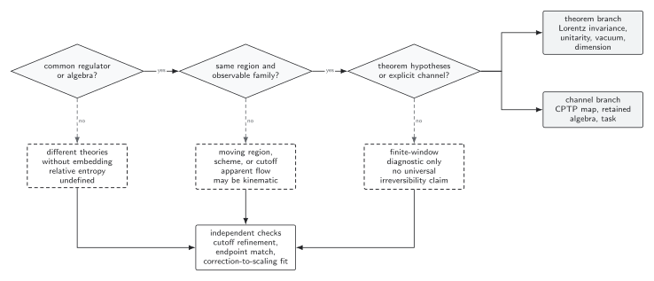
Independent validity gates. Passing the theorem gate does not produce a channel, and identifying a channel establishes data processing but not a dimension-specific RG theorem. Quantitative recovery additionally requires a well-defined finite loss and the hypotheses of a stated remainder theorem. A finite crossover or response metric has its own error and prescription controls. Failure of a gate narrows the conclusion rather than turning every observed trend into universal irreversibility. Schematic and not to scale.

When relative entropies are infinite, the formal difference

$$\Delta_D=D(\rho\Vert\sigma)-D(\mathcal N\rho\Vert\mathcal N\sigma)$$

is not an $\infty-\infty$ number. One must instead work in a setting where both terms and the remainder theorem are defined, or formulate the comparison by a regulated limit whose convergence is demonstrated. This small-looking check is representative of the chapter: the mathematical object, the physical scale path, and the licensed conclusion must all match.

References

• Casini, Horacio, and Marina Huerta. “A c-Theorem for the Entanglement Entropy.” Journal of Physics A: Mathematical and Theoretical 40 (2007): 7031–7036. DOI.
• Casini, Horacio, and Marina Huerta. “On the RG Running of the Entanglement Entropy of a Circle.” Physical Review D 85 (2012): 125016. DOI.
• Casini, Horacio, Eduardo Testé, and Gonzalo Torroba. “Markov Property of the Conformal Field Theory Vacuum and the a Theorem.” Physical Review Letters 118 (2017): 261602. DOI.
• Komargodski, Zohar, and Adam Schwimmer. “On Renormalization Group Flows in Four Dimensions.” Journal of High Energy Physics 2011, no. 12 (2011): 099. DOI.

Further reading

• Liu, Hong, and Mark Mezei. “A Refinement of Entanglement Entropy and the Number of Degrees of Freedom.” Journal of High Energy Physics 2013, no. 4 (2013): 162. DOI.