Local Measurements, Detectors, and Instruments

A local measurement in quantum field theory is a physical protocol, not merely an observable with a position label. A probe must be prepared, coupled to a smeared field in a declared spacetime region, read out, and discarded or retained. The complete protocol determines an instrument: outcome probabilities together with the conditional and nonselective changes of the field state. This chapter builds that dictionary and then asks three separate questions of every proposal: Does the detector response have a controlled regulator? Is the induced operation local in the causal sense? Does the recorded data justify the advertised inference?

The scope is measurement structure in flat-spacetime QFT. Accelerated and curved-spacetime detector phenomenology is developed in the next volume, while the local-covariant scattering framework is taken further in the mathematical-QFT volume.

Helpful background. Local regions and their algebras supplies the net-of-algebras language, and restricted states explains why a sharp local algebra generally has no density matrix of its own. Review relativistic causality and operator-valued distributions before taking pointlike or instantaneous limits. The open-system routes on influence functionals and Lindblad field dynamics help distinguish a finite intervention from a continuous reduced-dynamics approximation.

From a local coupling to a field instrument

Let the field system have algebra $\mathcal A$ and the probe have algebra $\mathcal B$. Prepare a field state $\omega$ and a probe state $\sigma$. The uncoupled preparation is $\omega\otimes\sigma$. A coupling supported in a compact spacetime region $K$ produces a scattering automorphism $\Theta$ of the joint algebra. The convention used here is that an outgoing observable is pulled back by $\Theta$, so the outgoing joint state is $\Theta^*(\omega\otimes\sigma)$.

Suppose the probe readout is described by a POVM $E$, and $E_X\in\mathcal B$ is the effect associated with an outcome set $X$. The induced field effect is

$$\varepsilon_\sigma(E_X) = (\operatorname{id}\otimes\sigma) \!\left[\Theta(\mathbf 1\otimes E_X)\right].$$

It reproduces the actual probe probability in every field state:

$$p_\omega(X) =\omega\!\left(\varepsilon_\sigma(E_X)\right) =(\omega\otimes\sigma) \!\left[\Theta(\mathbf 1\otimes E_X)\right].$$

Thus a probe effect becomes a field effect only after the probe preparation and the interaction have been specified. The induced-observable map $\varepsilon_\sigma$ is completely positive and unital, but it is generally neither injective nor multiplicative. These properties, and the localization of the induced effect in any connected causally convex region containing $K$, are Fewster and Verch 2020, Theorems 3.2–3.3.

Probabilities are only half of a measurement. Define the Heisenberg-picture operation

$$\mathcal I_X^*(A) =(\operatorname{id}\otimes\sigma) \!\left[\Theta(A\otimes E_X)\right], \qquad A\in\mathcal A.$$

Its dual sends the incoming field state to the subnormalized branch

$$\mathcal I_X(\omega)(A)=\omega\!\left(\mathcal I_X^*(A)\right), \qquad \mathcal I_X(\omega)(\mathbf 1)=p_\omega(X).$$

If $p_\omega(X)>0$, the conditional field state is

$$\omega_X(A)= \frac{\mathcal I_X(\omega)(A)}{p_\omega(X)}.$$

The family $X\mapsto\mathcal I_X$ is the instrument. Its nonselective operation is $\mathcal I_\Omega=\sum_x\mathcal I_x$ for a discrete readout, or the corresponding measure over outcomes. It is trace preserving, equivalently $\mathcal I_\Omega^*(\mathbf 1)=\mathbf 1$. A conditional state is undefined when its conditioning event has zero probability; when the probability is merely tiny, statistical and calibration errors are amplified.

These distinctions are easy to miss, so the chapter uses one finite-dimensional calibration target repeatedly. Let a qubit system interact with a qubit probe prepared in $|0\rangle$ through

$$U_\theta= \exp\!\left(-\frac{i\theta}{2}\,\sigma_z\otimes\sigma_y\right), \qquad 0\leq\theta\leq\frac{\pi}{2},$$

and measure the probe in the $\sigma_x$ basis. The two Kraus operators are

$$M_\pm=\frac{1}{\sqrt 2} \left( \cos\frac{\theta}{2}\,\mathbf 1 \pm \sin\frac{\theta}{2}\,\sigma_z \right),$$

so

$$E_\pm=M_\pm^\dagger M_\pm =\frac12\left(\mathbf 1\pm\sin\theta\,\sigma_z\right), \qquad E_++E_-=\mathbf 1.$$

For an input Bloch vector $\boldsymbol r$, the outcome probabilities are $p_\pm=(1\pm\sin\theta\,r_z)/2$. If the outcome is ignored, the channel is

$$\mathcal E_\theta(\rho) =\cos^2\frac{\theta}{2}\,\rho +\sin^2\frac{\theta}{2}\,\sigma_z\rho\sigma_z,$$

which maps $(r_x,r_y,r_z)$ to $(\cos\theta\,r_x,\cos\theta\,r_y,r_z)$. At $\theta=0$ the record is uninformative and the system is undisturbed; at $\theta=\pi/2$ the effects become the projectors onto $\sigma_z$ and the nonselective channel fully dephases that basis. Replacing $M_\pm$ by $V_\pm M_\pm$ for arbitrary outcome-dependent unitaries $V_\pm$ leaves $E_\pm$ and every immediate outcome probability unchanged while altering later statistics. This is the simplest explicit proof that a POVM does not determine its instrument.

The qubit calculation certifies algebraic identities, not spacetime locality. A field implementation must additionally state the support, switching, smearing, energy budget, and causal action of the full system–probe coupling.

Inspect those dependencies from left to right in the protocol map. Its lower panel then separates a shared field preparation from two spacelike coupling supports and shows that the classical records meet only in their common future.

A supported interaction, a calibrated probe readout, and the induced field instrument are distinct stages. Support and regulator tests belong to the coupling; complete positivity, normalization, and disturbance belong to the instrument; causal and statistical tests delimit the final claim. For two spacelike couplings, a common input may correlate the records, but there is no causal arrow between the supports; the records can be compared only in their common future. Schematic and not to scale.

A route through the chapter

The first four pages construct detector response without treating a click as a primitive particle count. Operational locality starts from spacetime protocols and causal dependency graphs. Localized detector models derives the response of a smeared two-level probe. Switching and smearing shows why the order of pointlike and sudden-switching limits matters. Detector responses and field observables then compares a trajectory-dependent response with field observables and particle interpretations.

The middle four pages build the operation. System–probe scattering derives induced effects and instruments from a compact coupling. Local instruments separates an outcome effect from its update map. Causal channels tests how two localized operations compose. Selective operations and postselection distinguishes unconditional statistics, locally conditioned statistics, and data available only after a classical record arrives.

The final four pages test what the operation licenses. Energy, noise, and backreaction separates detector excitation, switching work, field-energy change, and readout noise. Spacelike joint measurements compares the two orders of composition. Witnesses and tomography limits explains what finite moments can and cannot certify. Detector and instrument validation closes the loop with analytic benchmarks, numerical convergence, null tests, and adversarial failure seeds.

Model-to-claim comparison

The comparison table is a routing device, not a ranking. “Local” means that the action of the complete operation on observables in the causal complement is controlled. A localized Hamiltonian density, a local-looking Kraus representation, or complete positivity by itself is not that control.

Measurement models compared by physical support, readout, channel properties, energetic account, causal test, calibration target, and falsification condition.

Model or claim	Interaction support	Switching or smearing	Recorded and induced object	Instrument check	Energy and noise account	Causal composition test	Calibration target	What falsifies the advertised use?
Smeared two-level detector	Declared worldtube	Smooth switching χ and spatial profile F	Probe excitation or probe POVM; sampled field two-point function	Positivity and perturbative normalization	Gap energy, switching work, response variance, and neglected higher orders	Separate the receiver from the full support, including tails	Vacuum and one-particle response with analytic limiting cases	A persistent acausal response after support tails and numerical error are bounded
Compact scattering probe	Compact coupling region K	Smooth coupling coefficient with support in K	Probe effect and induced field effect	Complete positivity, normalization, and normality where required	Probe preparation, coupling work, and field backreaction	Factorize two causally ordered couplings; reverse spacelike ones	Exactly solvable linear model or a controlled perturbative expansion	Order dependence for genuinely spacelike, disjoint coupling regions
Gaussian unsharp field instrument	Support of the smeared quadrature and apparatus coupling	Finite resolution and a stated test function	Continuous outcome and effect density	Complete positivity, normalization, and operator-domain control	Added readout noise and conjugate disturbance	Identity action on the causal complement for the nonselective map	Finite-mode Gaussian channel with known moments	A claimed sharp limit with divergent energy or uncontrolled domains
Selective or postselected protocol	Physical coupling plus storage and transport of a classical record	Same regulator as the nonselective protocol	Subnormalized outcome branch	Positive outcome weight and normalized branch only when the weight is nonzero	Success probability, repetitions, and communication cost	Compare unconditional, locally available, and record-conditioned statistics	Explicit joint distribution including the record	A remote change appears only after unavailable outcome sorting
Spacelike joint measurement	Two disjoint coupling regions	Each support and every tail checked separately	Pair of local outcomes and the composite instrument	Complete positivity of each branch and normalization of the sum	Separate apparatus accounts plus any shared control	Compose the two instruments in both orders on a spanning observable set	Finite-dimensional or Gaussian model with exact reversed-order equality	Commuting effects but order-dependent state updates
Witness or partial tomography	Calibrated setting supports and a declared state class	Bandwidth, mode functions, and resolution recorded	Selected correlators, covariance entries, or witness value	Physical reconstructed data and valid confidence region	Shot noise, truncation, drift, and model discrepancy	Check setting independence and common support assumptions	Synthetic states inside and outside the claimed class	A counterexample shares all measured data but reverses the inference

Three independent validity questions

Does the response describe the declared detector?

At leading nontrivial order, a linearly coupled detector response is a switched and smeared two-point function. Schematically,

$$P_{g\to e}^{(2)} =\lambda^2 \int d\tau\,d\tau'\, \chi(\tau)\chi(\tau') e^{-i\Omega(\tau-\tau')} W_F(\tau,\tau'),$$

where $\chi$ is the switching, $F$ is the spatial profile hidden in $W_F$, $\Omega$ is the detector gap, and $\lambda$ is the coupling. A point field is a distribution, so $\chi$, $F$, the trajectory, and the order of limits are part of the observable being calculated. Smooth compact switching and smearing give a well-defined physical protocol; a formal sudden or pointlike limit needs its own convergence argument. Schlicht 2004, Eqs. (3)–(7) and §§3–4 demonstrates concretely how a regulator that is harmless in one frame can give an unphysical nonstationary response for an accelerated detector, and how finite detector size supplies a physical regularization.

Response validation therefore includes an off-coupling null test, positivity, perturbative scaling with $\lambda^2$, convergence under grid refinement, a benchmark state with known response, and separate variation of switching and spatial width. A detector click is evidence about this response functional; it is not automatically a measurement of a basis-independent global particle number.

Is the operation local in the causal sense?

Complete positivity says that the operation remains positive when an arbitrary spectator ancilla is appended. It does not specify where the operation acts. Locality is instead tested on the net of field algebras and on the scattering map. For a nonselective coupling in $K$, an observable $A$ localizable in the causal complement obeys

$$\mathcal I_\Omega^*(A)=A.$$

For two probes with appropriately causally ordered compact coupling regions, the corresponding instruments compose in causal order. When the regions are causally disjoint, the two orders agree; this is Fewster and Verch 2020, Theorem 3.5. A useful numerical test does not merely compare the POVM effects. It applies both composite superoperators to a spanning set of observables or states, because commuting effects can conceal noncommuting updates.

Does the data license the inference?

Postselection can change correlations conditioned on an outcome without enabling a remote observer who lacks that outcome to detect any change. For $A$ in the causal complement of $K$, the selective branch has the form

$$\mathcal I_X(\omega)(A) =\omega\!\left(A\,\varepsilon_\sigma(E_X)\right),$$

so the normalized conditional value can differ from $\omega(A)$ when the incoming state is correlated. The nonselective value remains unchanged. The classical record and the time at which it becomes accessible therefore belong to any signaling claim. In the multi-probe setting, the explicit no-signaling result is Bostelmann, Fewster, and Ruep 2021, Theorem 2 and Eqs. (11)–(12).

Inference validity also limits witnesses and tomography. Second moments determine a Gaussian state but not a general non-Gaussian state. A finite collection of settings can certify only the property whose witness theorem, state class, calibration, and confidence region have actually been checked. An adversarial state sharing the measured moments is often more informative than another fit inside the assumed model.

The failure map places these three questions side by side. Passing one branch does not certify the other two.

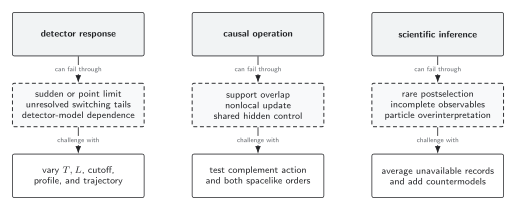
Detector-response validity, operation locality, and inference validity have different failure modes and different controls. Regulator convergence cannot prove causal composition; complete positivity cannot prove localization; and a causal instrument cannot make incomplete data tomographically complete. Schematic.

The strength and limits of the framework

The localized system–probe construction gives a disciplined route from dynamics to effects and instruments. It explains why a probe observable outside the causal influence of the coupling induces only a trivial multiple of the identity, why a nonselective localized intervention leaves causally disjoint observables unchanged, and why spacelike instruments can compose consistently. It also removes any need to imagine an instantaneous global collapse surface.

It does not say that every abstract completely positive instrument has a compactly supported realization in a QFT. On a general von Neumann algebra, implementability by a measuring process requires extension and normality properties; the normal extension property is defined and related to measuring processes in Okamura and Ozawa 2016, Definition III.3, Theorem III.4, and Corollary III.5. Nor does the framework rescue a protocol whose apparatus is silently nonlocal. The lesson of “impossible measurement” scenarios is that an operation capable of the advertised task may require an apparatus with impossible localization, not that QFT permits superluminal control.

A publication-quality claim should therefore ship with six items: the coupling and its support; the switching, smearing, and regulator; the probe preparation and readout; the full instrument rather than only its effects; the energy, noise, and perturbative account; and a failure test targeted at the specific conclusion. The pages that follow make each item executable on a small benchmark before returning to the field-theoretic statement.

Exercises

1. Verify the unsharp qubit instrument. Starting from $U_\theta$ and a probe in $|0\rangle$, derive $M_\pm$, $E_\pm$, and the nonselective Bloch-vector map. Check the two limits $\theta=0$ and $\theta=\pi/2$.

Solution

Because $\sigma_y|0\rangle=i|1\rangle$,

$$U_\theta|\psi,0\rangle =\cos\frac\theta2|\psi,0\rangle +\sin\frac\theta2\,\sigma_z|\psi,1\rangle.$$

Projection onto $|\pm_x\rangle=(|0\rangle\pm|1\rangle)/\sqrt2$ gives

$$M_\pm=\langle\pm_x|U_\theta|0\rangle =\frac{1}{\sqrt2} \left(\cos\frac\theta2\,\mathbf1 \pm\sin\frac\theta2\,\sigma_z\right).$$

Squaring gives $E_\pm=(\mathbf1\pm\sin\theta\,\sigma_z)/2$ and $E_++E_-=\mathbf1$. Adding the two branches cancels the cross terms:

$$\sum_\pm M_\pm\rho M_\pm^\dagger =\cos^2\frac\theta2\rho +\sin^2\frac\theta2\sigma_z\rho\sigma_z.$$

Conjugation by $\sigma_z$ reverses the $x$ and $y$ Bloch components, so they are multiplied by $\cos^2(\theta/2)-\sin^2(\theta/2)=\cos\theta$, while $r_z$ is unchanged. At $\theta=0$ both outcomes have probability $1/2$ and the channel is the identity. At $\theta=\pi/2$ the effects are the two $\sigma_z$ projectors and the channel removes all $\sigma_z$-basis coherence.

2. Separate conditioning from signaling. Let a localized two-outcome instrument act in region $K$, and let $A$ be an observable in the causal complement. Explain how $\omega_X(A)$ can differ from $\omega(A)$ while an observer near $A$ cannot use the protocol to receive a signal from $K$.

Solution

The selective numerator is $\mathcal I_X(\omega)(A)=\omega(A\varepsilon_\sigma(E_X))$. If the initial state correlates $A$ with the induced effect, division by $p_\omega(X)$ changes the conditional expectation. But the remote observer cannot sort trials by $X$ until the classical record is delivered. Without that record the relevant operation is nonselective, and locality gives

$$\mathcal I_\Omega(\omega)(A)=\omega(A).$$

The conditional correlation is real, but it is not locally accessible control. A signaling test must compare the unconditional distributions available at the receiver before any outcome message arrives.

3. Diagnose a failed certification. Two nominally spacelike devices have commuting POVM effects, and a simulation finds identical local outcome probabilities in both orders. Is that enough to certify a spacelike joint measurement? Give a stronger test.

Solution

No. Effects determine immediate probabilities but not the state updates. Outcome-dependent unitaries can leave every effect unchanged while making the two instruments fail to commute. The stronger test first verifies that the complete coupling supports, including switching and smearing tails, are spacelike. It then composes the two selective and nonselective superoperators in both orders on a spanning set of states or observables and requires agreement within a stated analytic or numerical tolerance. A shared controller or hidden record channel must also be included in the support analysis.

References

• Bostelmann, Henning, Christopher J. Fewster, and Maximilian H. Ruep. “Impossible Measurements Require Impossible Apparatus.” Physical Review D 103 (2021): 025017. DOI. Open PDF.
• Fewster, Christopher J., and Rainer Verch. “Quantum Fields and Local Measurements.” Communications in Mathematical Physics 378 (2020): 851–889. DOI. Open PDF.
• Okamura, Kazuya, and Masanao Ozawa. “Measurement Theory in Local Quantum Physics.” Journal of Mathematical Physics 57 (2016): 015209. DOI. Open PDF.
• Schlicht, Sebastian. “Considerations on the Unruh Effect: Causality and Regularization.” Classical and Quantum Gravity 21 (2004): 4647–4660. DOI. Open PDF.