Information-Measure Domain and Comparison Atlas

No single information measure ranks every QFT state, channel, and protocol. A quantity is admissible only when both its mathematical input and its operational question are defined on the declared algebra, support, resource set, and regulator prescription. The answer is therefore a domain-matching procedure, not a universal hierarchy.

Required background. Use Relative Entropy for QFT States for state and algebra conventions and Infinite-Dimensional and Energy-Constrained Channel Distances for channel resources. Helpful background. Hypothesis Testing and Asymptotic Distinguishability and Mutual Information and Regulator-Independent Correlations develop the main decision and correlation tasks.

The chapter’s canonical task-comparison table is the compact cross-check, and its machine-readable form preserves the same claim boundaries. This atlas explains how to use that comparison without silently changing the problem.

The data that define an information question

Before selecting a formula, write down eight pieces of information.

1. Object and question. Are the inputs a state pair, a channel pair, an algebra inclusion, a bipartite correlation problem, or a tripartite recovery problem? Is the goal testing, equal-prior discrimination, compression, correlation, recovery, or channel comparison?
2. Algebra, state order, and support. Which observables are accessible? Are the states normal on that algebra, which state is the reference, and does the ordered pair satisfy the support or absolute-continuity condition required by the result?
3. Error and smoothing. State the type-I tolerance, root- or squared-fidelity convention, smoothing metric and radius, normalization of nearby states, optimized argument, and logarithm base.
4. Copy and operation model. State the number of preparations, whether they are independent or correlated, and the allowed measurement or recovery maps.
5. Energy resource. Fix the physical Hamiltonian, numerical budget, systems counted, and whether an ancilla is an inert reference or an acted-on input.
6. Regulator and limits. Fix the ultraviolet and volume regulators, boundary or center prescription, detector smearing, and order of limits.
7. Output semantics. Say whether the result is an exact value, one-sided bound, theorem interval, asymptotic expansion, regulated estimate, or continuum theorem; include units and norm normalization.
8. Licensed conversions. Name the theorem that converts the chosen output into another quantity and check its hypotheses independently.

If a field needed by the definition is missing, the quantity is not yet defined. A valid singular branch is different: failed absolute continuity can make a relative entropy equal to $+\infty$. If only a conversion theorem fails, retain the base quantity and reject the conversion. Producing a precise decimal first and supplying the domain afterward reverses the logical order.

The structure map organizes the first decision. Inspect the branch point: state comparison, testing, correlation, recovery, and channel comparison do not share one optimization problem.

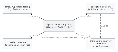
State comparison is not a single numerical ranking. Choose the branch from the decision task: regulated entropy, asymmetric reference comparison, one-shot or many-copy discrimination, correlation, recovery, or channel discrimination. Schematic.

Measure families and what their numbers mean

Regulated entropy versus intrinsic relative entropy

For a finite-dimensional regulator with a specified tensor factor $A$,

$$S(\rho_A)=-\operatorname{Tr}(\rho_A\log\rho_A)$$

is a well-defined entropy. In a continuum QFT, however, a sharp local algebra is typically type III and has no density matrix or trace of this kind. A lattice spacing, split inclusion, mode cutoff, or other type-I prescription creates a regulated quantity $S(\rho_A^{(a)})$; the answer must retain that prescription until a proved universal combination or controlled limit is extracted. The ultraviolet structure of subregion entropy is reviewed in Casini and Huerta 2009, §§ 2–3.

Araki relative entropy instead compares two normal states on one von Neumann algebra. It is asymmetric, may be infinite, and does not require a density matrix for the local algebra Araki 1976, Eqs. (1.1)–(1.2), p. 809. Use it for an intrinsic “state versus reference” question; do not call it the entropy of either state. Likewise, mutual information for separated regions can be intrinsic when a split or comparable hypothesis supplies a normal product reference and the resulting Araki relative entropy is finite. Separation alone proves neither condition: suitable nuclearity assumptions imply the split property in standard AQFT settings Fewster 2016, § 2, while finiteness is a further model-dependent result, as in the free-fermion vacuum Xu 2020, § 3, Corollary 3.7.

One-shot testing and smooth relative quantities

For density operators and an allowed effect $0\leq Q\leq I$, the hypothesis-testing divergence is

$$D_H^\varepsilon(\rho\Vert\sigma) =-\log\inf_{ \substack{0\leq Q\leq I\\ \operatorname{Tr}(Q\rho)\geq1-\varepsilon} } \operatorname{Tr}(Q\sigma).$$

It answers one asymmetric binary decision: keep the type-I error at most $\varepsilon$ and minimize the type-II error. The effect algebra and state order are part of the definition. A detector-restricted value is not the unrestricted value on the full field algebra.

Two related one-shot divergences are the support min-relative entropy and the max-relative entropy,

$$\begin{aligned} D_{\min}(\rho\Vert\sigma) &=-\log\operatorname{Tr}(\Pi_\rho\sigma),\\ D_{\max}(\rho\Vert\sigma) &=\inf\{\lambda\in\mathbb R:\rho\leq e^\lambda\sigma\}, \end{aligned}$$

where $\Pi_\rho$ is the support projection. For normalized states and the testing convention above, $D_H^0=D_{\min}$: the zero-error constraint forces $Q$ to contain $\Pi_\rho$. This identity does not equate their smoothed versions. For a purified-distance ball $\mathcal B_P^\varepsilon(\rho)$ of subnormalized states, one consistent convention is

$$\begin{aligned} D_{\min}^{\varepsilon,P}(\rho\Vert\sigma) &=\sup_{\widetilde\rho\in\mathcal B_P^\varepsilon(\rho)} D_{\min}(\widetilde\rho\Vert\sigma),\\ D_{\max}^{\varepsilon,P}(\rho\Vert\sigma) &=\inf_{\widetilde\rho\in\mathcal B_P^\varepsilon(\rho)} D_{\max}(\widetilde\rho\Vert\sigma). \end{aligned}$$

The superscript matters. A trace-distance ball with the same numerical radius is a different feasible set, and normalized versus subnormalized smoothing changes boundary terms. Support leakage makes unsmoothed $D_{\max}$ infinite, whereas smoothing over subnormalized states can even make a smooth max-relative entropy negative. Relative $D_{\min/\max}$ also differs from conditional $H_{\min/\max}$. Use a smooth quantity when a one-shot coding, extraction, or resource theorem is formulated in that same convention—not merely because the system is finite. Datta 2009, Definitions 1–2 and 4, pp. 2818 and 2823 and Tomamichel and Hayashi 2013, Definitions 2–5 and Eq. (6), pp. 7697–7700 illustrate why conventions must be translated explicitly.

Relative-entropy variance is a second-order coefficient

For an ordered density-operator pair with $\operatorname{supp}\rho\subseteq\operatorname{supp}\sigma$ and finite logarithmic second moment,

$$V(\rho\Vert\sigma) =\operatorname{Tr}\rho \left( \log\rho-\log\sigma-D(\rho\Vert\sigma) \right)^2.$$

It is not a new distance. It controls the $\sqrt n$ correction in an independent-copy testing problem. In the finite-dimensional iid setting, for fixed $0<\varepsilon<1$ and the present state order,

$$D_H^\varepsilon (\rho^{\otimes n}\Vert\sigma^{\otimes n}) =nD(\rho\Vert\sigma) +\sqrt{nV(\rho\Vert\sigma)}\,\Phi^{-1}(\varepsilon) +O(\log n),$$

with a separate degenerate branch when $V=0$. Li 2014, Theorems 2 and 5, pp. 174–176 and 183–184 gives the second-order theorem and finite-sample bounds. Correlated spatial regions of one QFT state are not automatically copies, finite mean energy does not guarantee the logarithmic moment, and the displayed asymptotic expression is not a one-copy bound.

Fidelity, recovery, and channel distance

This site uses root fidelity

$$F(\rho,\sigma)=\left\lVert\sqrt\rho\sqrt\sigma\right\rVert_1,$$

so a source using transition probability reports $F^2$. With $T(\rho,\sigma)=\tfrac12\lVert\rho-\sigma\rVert_1$, the Fuchs–van de Graaf inequalities read

$$1-F(\rho,\sigma) \leq T(\rho,\sigma) \leq\sqrt{1-F(\rho,\sigma)^2}.$$

These are bounds for the same state pair on the same algebra, not a conversion between unrelated experiments Fuchs and van de Graaf 1999, Theorem 1 and Eq. (46), p. 1223.

For a declared tripartition, conditional mutual information can certify the existence of a good recovery map. In the finite-dimensional convention used here,

$$I(A{:}C\mid B)_\rho \geq -2\log F\!\left( \rho_{ABC}, \mathcal R_{B\to BC}(\rho_{AB}) \right).$$

This is the finite-dimensional recovery theorem Fawzi and Renner 2015, Theorem 5.1. Its conclusion is an existence guarantee within the theorem’s channel class. If the physical problem permits only a narrower class, the displayed theorem does not by itself certify that restricted optimum. Nor does it make a recovery map geometrically local, gauge covariant, computationally feasible, energy bounded, or stable in a continuum limit. Universal rotated-Petz recovery and its support hypotheses are given by Junge et al. 2018, Theorem 2.1 and Remark 2.2, pp. 2961–2963.

Finally, channel discrimination requires a channel norm. For an infinite-dimensional input, the ordinary diamond norm can treat arbitrarily energetic states as free resources. An energy-constrained diamond norm fixes a positive Hamiltonian $G_A$, a budget $E$, the physical input, and the role of the reference. Its number answers that one resource-bounded channel task; it is not evidence of unconstrained uniform closeness Shirokov 2018, Eq. (2) and Proposition 3; arXiv v2, pp. 5–7.

Translations require a theorem

Several useful bridges are licensed, but each carries hypotheses.

• Relative entropy to trace norm. With natural logarithms, quantum Pinsker gives $D(\rho\Vert\sigma)\geq\tfrac12\lVert\rho-\sigma\rVert_1^2$ for one common state pair. It supplies a one-sided bound, not an equality or a ranking of different pairs.
• Fidelity to trace distance. Use the Fuchs–van de Graaf interval above and first translate root versus squared fidelity.
• Zero-error testing to min-relative entropy. $D_H^0=D_{\min}$ holds for the definitions on this page. Smooth variants require the same ball, normalization, and shifted error parameters as the cited theorem.
• One shot to asymptotic rate. Stein’s limit Ogawa and Nagaoka 2000, Theorems 2–3 and Corollary 1, pp. 2429–2432 and the $V$ correction require a declared iid or otherwise theorem-covered sequence. “Many degrees of freedom” is not the same assumption.
• Conditional information to recovery. A small conditional mutual information guarantees good recovery only in the theorem’s channel class and domain. A stricter physical class can have a smaller optimum.
• Energy-bounded to unconstrained channels. There is no such promotion without an additional uniform-energy argument. Convergence for every fixed $E$ is a family of bounded-resource statements.

If a proposed conversion is absent from this list, return to the task definition rather than treating two quantities as interchangeable units.

Four QFT decisions

The following cases execute the selection procedure. The point is not just to name a measure, but to state why it is admissible and what the result can mean.

A vacuum region

Take the $1+1$-dimensional free massless scalar, the interval $A=(-R,R)$, the vacuum $\omega_0$, and a normal coherent excitation $\omega_f$. At $t=0$, choose smooth compactly supported classical data

$$F(x)= \begin{cases} A\exp[-x^2/(r^2-x^2)], & |x|<r,\\ 0, & |x|\geq r, \end{cases} \qquad G(x)=0.$$

On the interval algebra, with the state order $\omega_f\Vert\omega_0$, the exact modular-energy formula is

$$S_A(\omega_f\Vert\omega_0) =2\pi\int_{-R}^{R} \frac{R^2-x^2}{2R}\,T_{00}(x)\,dx, \qquad T_{00}=\frac{F'(x)^2+G(x)^2}{2}.$$

For $R=1$, $r=1/2$, and $A=1$, the reproducible interval record gives

$$S_A(\omega_f\Vert\omega_0)=8.415964488746008\ \text{nats}.$$

The continuum formula and independent high-precision quadratures support this value; the harmonic-chain rows are empirical regulator-convergence checks, not statistical samples or rigorous continuum error bars. Smoothness, localization, normality, the quadratic-form domain, the interval algebra, and the state order are theorem-level inputs Bostelmann, Cadamuro, and Del Vecchio 2022, Theorem 2.13 and Eq. (2.32) Garbarz and Palau 2023, § IV.B.2, Eqs. (91) and (95), p. 125016-10. A changed algebra or failed form-domain condition rejects this formula. Failed absolute continuity instead gives the legitimate extended value $+\infty$.

If the question asks for “the entropy of the sharp region,” stop: the type-III algebra has no reduced density matrix. A type-I regulator defines a different, cutoff-dependent quantity.

Finite-copy bosonic discrimination

Consider one detector-selected bosonic wavepacket mode with thermal mean occupation $N=1/2$. The ordered states are

$$\rho=\mathsf D(1)\tau_{1/2}\mathsf D(1)^\dagger, \qquad \sigma=\tau_{1/2},$$

prepared independently $n$ times. Restrict the receiver to homodyne measurement of $q=(a+a^\dagger)/\sqrt2$ and set the type-I tolerance to $\varepsilon=0.1$. The induced laws are $\mathrm N(\sqrt2,1)$ under $\rho$ and $\mathrm N(0,1)$ under $\sigma$. At $n=4$, the exact Gaussian threshold test in the operational benchmark gives

$$\beta_{0.1}=0.0609466278214072, \qquad D_{H,q}^{0.1}=-\log\beta_{0.1} =2.7977567515516975\ \text{nats}.$$

The same record has the homodyne coefficients $D_q=1$ nat and $V_q=2$ nats$^2$, while unrestricted quantum relative entropy gives $D=\log3$ and $V=2(\log3)^2$. These are asymptotic diagnostics. In particular,

$$nD_q+\sqrt{nV_q}\,\Phi^{-1}(0.1) =0.3752247902527075 \qquad (n=4),$$

which is far below the exact $D_{H,q}^{0.1}$. The second-order expansion is not a finite-blocklength bound. Rotating to a blind quadrature, correlating the preparations, changing the state with the cutoff, or allowing finite $D$ but infinite $V$ removes at least one claim. The exact finite-$n$ number survives only for the declared homodyne test; the unrestricted collective quantum test is a different optimization.

Gauge-sector recovery

An exact finite regulated model makes the output semantics visible. Let

$$\mathcal H=\bigoplus_q (\mathcal H_{L,q}\otimes\mathcal H_{G,q}), \qquad \mathcal A=\bigoplus_q \bigl(\mathcal B(\mathcal H_{L,q})\otimes I_{G,q}\bigr).$$

Here $q$ labels superselection sectors, $L$ contains the observable logical factor, and $G$ is invisible to $\mathcal A$. In a basis $\{|j_q\rangle\}$ of $\mathcal H_{G,q}$, define

$$K_{qj}=I_{L,q}\otimes|0_q\rangle\langle j_q|P_q, \qquad \mathcal N(\rho)=\sum_{q,j}K_{qj}\rho K_{qj}^\dagger,$$

where $P_q$ projects onto sector $q$. The Kraus operators are complete. For every $X\in\mathcal A$,

$$\mathcal N^\dagger(X) =\sum_{q,j}K_{qj}^\dagger X K_{qj} =X.$$

Thus the observable algebra is exactly preserved: its algebra-correction error is zero. This is the Heisenberg-picture correction criterion Bény, Kempf, and Kribs 2007, Eqs. (1), (3)–(5), and Theorem 2, pp. 100502-1–100502-2.

Now choose a representative in one sector whose $G$ factor is $|1_q\rangle$. The channel replaces it by $|0_q\rangle$. On the extended Hilbert space the input and output therefore have root fidelity $0$, half trace distance $1$, and trace-norm difference $2$. There is no contradiction: exact recovery of $\mathcal A$ and recovery of the full representative state are different claims, and the latter metric is representation dependent when $G$ is not observable.

Enlarging $\mathcal A$ by a $G$ observable, erasing or mixing the sector label $q$, or changing the electric/magnetic center changes the problem and can destroy exact correction. The sector decomposition and dependence on algebra choice are discussed by Casini, Huerta, and Rosabal 2014, §§ II–IV. Continue to Gauge Subregions, Centers, and Algebra Choices and Covariant Channels and Symmetry-Respecting Recovery for the physical operation class.

An energy-constrained channel

Let $G=\sum_{m\geq0}m|m\rangle\langle m|$, let $P_N$ project onto levels $0$ through $N$, and define the trace-preserving cutoff-and-replace channel

$$\mathcal C_N(\rho) =P_N\rho P_N +\operatorname{Tr}(Q_N\rho)|0\rangle\langle0|, \qquad Q_N=I-P_N.$$

For the identity channel $\mathcal I$ and inputs satisfying $\operatorname{Tr}(G\rho_A)\leq E$, set $\delta=\min\{1,E/(N+1)\}$. The two-level witness and gentle-projection estimate give

$$2\sqrt\delta \leq \lVert\mathcal I-\mathcal C_N\rVert_{\diamond,E,G} \leq \min\{2,2\sqrt\delta+\delta\}.$$

For the stored choice $E=2$ and $N=31$, $\delta=1/16$, and the recovery and channel benchmark gives

$$0.5 \leq \lVert\mathcal I-\mathcal C_{31}\rVert_{\diamond,2,G} \leq0.5625.$$

With equal priors, the corresponding one-use success probability lies in $[0.625,0.640625]$. These widths are theorem gaps between a coherent two-level witness and a gentle-projection upper bound, not numerical uncertainty. The inert reference is unrestricted, while any auxiliary mode entering the device belongs to the physical channel input and its energy accounting.

Keeping the symbol $E$ while replacing $G$ by $G_N=G/(N+1)$ admits increasingly energetic number states into the feasible set. That sequence compares different resource theories, so it cannot establish convergence in one fixed energy-constrained norm.

Four QFT problems and the strongest admissible output.

Problem	Primary quantity	Must be fixed	Reject or downgrade when
Vacuum region	Araki relative entropy: 8.415964488746008 nats for the declared coherent profile	local algebra, state order, form domain, profile, continuum formula	the algebra or form-domain hypotheses change; a sharp-region entropy is requested without a regulator
Finite-copy bosonic test	homodyne DH0.1=2.7977567515516975 nats at n=4	state pair, ε, homodyne algebra, iid copies, log base	the detector, preparation sequence, support, or variance hypothesis changes
Gauge-sector recovery	zero algebra-correction error, despite maximal full-representative state error	observable algebra, center, sector action, and output metric	the algebra gains a G observable or the channel erases or mixes q
Bosonic channel cutoff	energy-constrained diamond-norm interval [0.5,0.5625] at E=2, N=31	physical input, fixed G, E, ancilla, cutoff channel	the Hamiltonian or input resource changes with the cutoff

Stop conditions before computation

Apply these checks in order. The validity map shows the same logic spatially; inspect the failure exits rather than following only the central path.

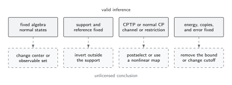
Before comparing numbers, verify that the algebras, supports, channel conventions, logarithms, energy sets, regulators, and operational classes match. A measure evaluated outside its domain is not rescued by a precise numerical value. Schematic.

The following table distinguishes a quantity that is undefined, a legitimate singular value, a failed conversion, and a genuinely changed task.

Adversarial inputs and the strongest statement that survives.

Input mutation	Failed hypothesis	Rejected output or conversion	Strongest surviving claim
Feed a sharp type-III region to the trace-entropy formula	No type-I density matrix or trace was specified	Reject the local von Neumann entropy	An algebraic relative entropy may still be intrinsic for a normal state pair
Change the observable algebra or gauge center	The two inputs no longer live on the same declared algebra	Reject the old comparison and its recovery claim	Restrict both states to one common algebra and pose the new problem explicitly
Let supp ρ extend outside supp σ	Absolute continuity needed for finite D and V	Reject a finite relative entropy and every finite-variance expansion	Return D(ρ‖σ)=+∞; a compatible finite-copy testing problem can remain defined
Give ε but no smoothing metric or normalization class	The optimization ball is unspecified	Reject the smooth min/max number	The unsmoothed divergence can survive if its own domain is complete
Replace iid copies by correlated repetitions	The tensor-power sequence used by Stein and second-order theorems is absent	Reject the iid rate and Gaussian correction	Define a fixed-n test on the actual joint state, or cite a theorem for that sequence
Insert V=∞ or V=0 into a nondegenerate Gaussian formula	The hypothesis 0<V<∞ fails	Reject the displayed √n correction	The first-order relative entropy can remain finite; analyze the exceptional branch separately
Quote “fidelity 0.9” without saying root or squared	The output convention is missing	Reject every numerical trace-distance conversion	The source result survives only after its convention is identified
Use a recovery map outside the allowed physical class	The map violates the algebra, normality, complete-positivity, symmetry, or support condition	Reject it as a feasible physical recovery	An unrestricted existence theorem survives within its own channel class
Infer locality, covariance, or energy feasibility from small conditional information	The recovery theorem does not supply that extra structure	Reject the added physical interpretation	Retain only existence and the theorem’s stated fidelity guarantee
Omit or vary G, E, the acted-on input, or reference convention	The energy-constrained feasible set is not fixed	Reject the constrained channel distance	Specify one resource theory; otherwise this is a family of different tasks
Reorder or leave uncontrolled the regulator limits	No common continuum prescription was established	Reject the continuum value or convergence claim	Report the finite-regulator result and the controls actually performed

Fix the mathematical object. A state pair cannot be compared with a channel pair, and two restrictions to different algebras are not the same input. If the objects differ, report “different tasks.”

Check normality and support. If a density-operator divergence needs $\operatorname{supp}\rho\subseteq\operatorname{supp}\sigma$ and the inclusion fails, report $D=+\infty$ and do not manufacture a finite variance. If a sharp local algebra has no density matrix, replace the density-matrix entropy question by an algebraic comparison or add a regulator.

Freeze error and smoothing conventions. A purified-distance ball, trace-distance ball, normalized ball, and subnormalized ball define different optimizations. If the convention is absent, the smooth value is not reproducible.

Verify the sequence. Before using Stein, Chernoff, an asymptotic equipartition property, or a second-order expansion, identify independent preparations or cite a theorem for the actual correlated sequence. Spatial repetition inside one field state is not enough.

Verify the physical operation class. A recovery map must act on the declared algebra and obey required locality, covariance, charge, and sector constraints. An unrestricted theorem provides no automatic certificate for a stricter class.

Hold resources fixed. A cutoff-dependent Hamiltonian, changing detector bandwidth, or newly available auxiliary mode changes the feasible set. Report the comparison as regulator dependent rather than as convergence in a fixed norm.

Control the continuum limit. State which quantities converge, in what topology, and in what order the ultraviolet, volume, copy-number, and energy limits are taken. If only finite-regulator evidence exists, say so.

For complete operator-algebraic definitions and infinite-dimensional proofs, continue to Noncommutative Lp Spaces, Divergences, and Information Bounds. For the downstream choice among entanglement-specific measures, continue to Choosing an Entanglement Measure for the Physical Question.

Common pitfalls

Treating a bound as a conversion factor. Pinsker, Fuchs–van de Graaf, and recovery inequalities define allowed intervals. They do not let one replace the original task or infer the converse inequality without new hypotheses.

Calling every finite-sample quantity “one shot.” One shot describes a resource model, not merely a small value of $n$. A finite block can still have iid structure, memory, detector restrictions, or a task whose operational characterization uses a different quantity.

Using the most computable measure. Fidelity or a regulated entropy may be easy to calculate while answering the wrong question. Select the task first, then use computability to choose among admissible methods.

Hiding a changed domain in notation. Reusing $\varepsilon$, $E$, or the same subsystem letter does not keep the problem fixed when the smoothing metric, Hamiltonian, algebra, or center has changed.

Exercises

1. Sharp-region entropy or algebraic relative entropy?

A calculation of the coherent excitation above asks for both $S(\rho_A)$ and $S_A(\omega_f\Vert\omega_0)$ in the continuum. Which request is defined without adding a type-I regulator? What evidence supports the reported decimal, and what does not constitute a rigorous error bar?

Solution

The sharp interval has a type-III local algebra, so an intrinsic reduced density matrix $\rho_A$ and trace entropy $S(\rho_A)$ are unavailable. A lattice, split factor, or another declared type-I construction would define a regulated entropy, but its regulator dependence must remain visible.

The ordered pair of normal states on the same interval algebra does admit Araki relative entropy. For the smooth coherent data, the modular-energy theorem reduces it to the displayed continuum integral. High-precision evaluation of that integral, checked by independent quadratures, supports $8.415964488746008$ nats. The lattice-spacing, box-size, and grid-phase sweeps are valuable empirical convergence controls, but without a lattice-to-continuum remainder theorem their spread is not a rigorous uncertainty interval.

2. Reproduce the four-copy homodyne result

For the Gaussian laws $\mathrm N(\sqrt2,1)$ and $\mathrm N(0,1)$, accept $\rho$ when the sample mean $\bar q$ exceeds a threshold $t$. At $n=4$ and $\varepsilon=0.1$, derive $t$, $\beta_{0.1}$, and $D_{H,q}^{0.1}$.

Solution

Under $\rho$, $\bar q$ is normal with mean $\sqrt2$ and variance $1/n$. Saturating the type-I constraint gives

$$\varepsilon =\Pr_\rho(\bar q<t) =\Phi\!\left(\sqrt n\,(t-\sqrt2)\right),$$

so

$$t=\sqrt2+\frac{\Phi^{-1}(0.1)}{2} =0.7734377796007949.$$

Under $\sigma$, the type-II error is

$$\beta_{0.1} =\Pr_\sigma(\bar q\geq t) =\Phi\!\left(-\sqrt{2n}-\Phi^{-1}(0.1)\right) =0.0609466278214072.$$

Therefore $D_{H,q}^{0.1}=-\log\beta_{0.1}=2.7977567515516975$ nats. This is exact for the declared Gaussian outcome model, up to numerical evaluation of $\Phi$; it is not the unrestricted quantum optimum.

3. Algebra recovery versus representative-state recovery

For the gauge-sector channel, verify $\sum_{q,j}K_{qj}^\dagger K_{qj}=I$ and $\mathcal N^\dagger(X)=X$ for $X\in\mathcal A$. Then compare a state with $G$ factor $|1_q\rangle$ to its output.

Solution

Within sector $q$,

$$\sum_jK_{qj}^\dagger K_{qj} =I_{L,q}\otimes\sum_j|j_q\rangle\langle j_q| =P_q.$$

Summing over $q$ gives $I$. Write $X=\bigoplus_q(X_{L,q}\otimes I_{G,q})$. Then

$$\sum_jK_{qj}^\dagger X K_{qj} =X_{L,q}\otimes\sum_j|j_q\rangle\langle j_q|,$$

and the sector sum returns $X$. Hence every observable in $\mathcal A$ is preserved exactly.

For a state $\rho_L\otimes|1_q\rangle\langle1_q|$, the output is $\rho_L\otimes|0_q\rangle\langle0_q|$. The two supports are orthogonal in the $G$ factor, so their root fidelity is $0$, half trace distance is $1$, and trace-norm difference is $2$. The algebra cannot observe that factor, which is why zero algebra error and maximal representative-state error coexist.

4. The moving-Hamiltonian trap

For the cutoff-and-replace channel, prove $\operatorname{Tr}(Q_N\rho)\leq E/(N+1)$ when $\operatorname{Tr}(G\rho)\leq E$. Evaluate the certified norm and equal-prior success intervals for $E=2$, $N=31$. Why does replacing $G$ by $G/(N+1)$ invalidate a fixed-resource convergence claim?

Solution

On the omitted subspace, $G\geq(N+1)Q_N$. Taking the expectation value gives

$$E\geq\operatorname{Tr}(G\rho) \geq(N+1)\operatorname{Tr}(Q_N\rho),$$

which yields the tail bound. At $E=2$, $N=31$, one has $\delta=2/32=1/16$. Thus $2\sqrt\delta=0.5$ and $2\sqrt\delta+\delta=0.5625$. The constrained diamond norm lies in $[0.5,0.5625]$, so $p_{\mathrm{succ}}=1/2+\lVert\mathcal I-\mathcal C_N\rVert_{\diamond,E,G}/4$ lies in $[0.625,0.640625]$.

With $G/(N+1)$, however, the state $|N+1\rangle$ has energy one for every $N$ and remains feasible at a fixed numerical budget. The feasible sets therefore change with $N$; the resulting norms do not describe convergence on one fixed energy-bounded set.

References

• Araki, Huzihiro. “Relative Entropy of States of von Neumann Algebras.” Publications of the Research Institute for Mathematical Sciences 11 (1976): 809–833. DOI.
• Bény, Cédric, Achim Kempf, and David W. Kribs. “Generalization of Quantum Error Correction via the Heisenberg Picture.” Physical Review Letters 98 (2007): 100502. DOI.
• Bostelmann, Henning, Daniela Cadamuro, and Simone Del Vecchio. “Relative Entropy of Coherent States on General CCR Algebras.” Communications in Mathematical Physics 389 (2022): 661–691. DOI.
• Casini, Horacio, and Marina Huerta. “Entanglement Entropy in Free Quantum Field Theory.” Journal of Physics A: Mathematical and Theoretical 42 (2009): 504007. DOI.
• Casini, Horacio, Marina Huerta, and José Alejandro Rosabal. “Remarks on Entanglement Entropy for Gauge Fields.” Physical Review D 89 (2014): 085012. DOI.
• Datta, Nilanjana. “Min- and Max-Relative Entropies and a New Entanglement Monotone.” IEEE Transactions on Information Theory 55 (2009): 2816–2826. DOI.
• Fawzi, Omar, and Renato Renner. “Quantum Conditional Mutual Information and Approximate Markov Chains.” Communications in Mathematical Physics 340 (2015): 575–611. DOI.
• Fewster, Christopher J. “The Split Property for Quantum Field Theories in Flat and Curved Spacetimes.” Abhandlungen aus dem Mathematischen Seminar der Universität Hamburg 86 (2016): 153–175. DOI.
• Fuchs, Christopher A., and Jeroen van de Graaf. “Cryptographic Distinguishability Measures for Quantum-Mechanical States.” IEEE Transactions on Information Theory 45 (1999): 1216–1227. DOI.
• Garbarz, Alan, and Gabriel Palau. “Relative Entropy of an Interval for a Massless Boson at Finite Temperature.” Physical Review D 107 (2023): 125016. DOI.
• Junge, Marius, Renato Renner, David Sutter, Mark M. Wilde, and Andreas Winter. “Universal Recovery Maps and Approximate Sufficiency of Quantum Relative Entropy.” Annales Henri Poincaré 19 (2018): 2955–2978. DOI.
• Li, Ke. “Second-Order Asymptotics for Quantum Hypothesis Testing.” The Annals of Statistics 42 (2014): 171–189. DOI.
• Ogawa, Tomohiro, and Hiroshi Nagaoka. “Strong Converse and Stein’s Lemma in Quantum Hypothesis Testing.” IEEE Transactions on Information Theory 46 (2000): 2428–2433. DOI.
• Shirokov, M. E. “On the Energy-Constrained Diamond Norm and Its Application in Quantum Information Theory.” Problems of Information Transmission 54 (2018): 20–33. DOI.
• Tomamichel, Marco, and Masahito Hayashi. “A Hierarchy of Information Quantities for Finite Block Length Analysis of Quantum Tasks.” IEEE Transactions on Information Theory 59 (2013): 7693–7710. DOI.
• Xu, Feng. “Some Results on Relative Entropy in Quantum Field Theory.” Communications in Mathematical Physics 374 (2020): 1469–1482. DOI.