Operational Preparation Cost and Energy-Constrained Bounds

Abstract circuit length becomes a physical preparation cost only after gates are implemented by a bounded control Hamiltonian. Quantum speed limits then give task-dependent lower bounds involving distinguishability and available energy or generator variance, while an explicit control protocol gives an upper bound. Neither direction identifies a universal conversion factor between geometric complexity, elapsed time, and work.

Required background. What Task Does Complexity Answer? supplies the resource tuple.

Helpful background. Passivity, Work, and Information in QFT distinguishes energy change from extractable work. Energy Cost of Localization and Measurement supplies the spacetime and switching costs hidden by ideal local operations.

Control model and reachable paths

Let

$$H(t)=H_0+\sum_Iu_I(t)H_I, \qquad \lvert u_I(t)\rvert\leq u_I^{\max},$$

act on a regulated, finite-energy domain. The allowed controls $H_I$, amplitude and bandwidth bounds, spatial support, ancillary states, and noise define the reachable set. A gate path is physically implemented only if its tangent generators can be synthesized from these controls with a quantified error.

One possible physical cost is

$$R[u]=\int_0^Tdt\left( \alpha+\sum_Ic_I\lvert u_I(t)\rvert +\sum_{IJ}g_{IJ}u_I(t)u_J(t) \right),$$

where the constant term charges duration and the others charge amplitude or power-like resources. The coefficients have units and require calibration. Reparameterizing a geometric path changes $T$ and $R$ once amplitude bounds are imposed, even though a homogeneous geometric length is unchanged.

A speed-limit theorem with hypotheses

For a pure state obeying Schrödinger evolution under a self-adjoint $H(t)$ on a common domain, define the Fubini–Study angle

$$\mathcal L(\psi_0,\psi_T)=\arccos\lvert\langle\psi_0|\psi_T\rangle\rvert.$$

The Mandelstam–Tamm argument gives Mandelstam and Tamm 1945, pp. 249–254

$$\mathcal L(\psi_0,\psi_T) \leq\int_0^Tdt\,\Delta_{\psi(t)}H(t), \qquad T\geq\frac{\mathcal L}{\overline{\Delta H}},$$

where $\overline{\Delta H}=T^{-1}\int_0^T\Delta H(t)dt$. This is a distinguishability bound, not a circuit-complexity theorem. Equality requires the evolution to follow an appropriate geodesic in projective state space with the variance resource used efficiently. Mixed states, open dynamics, and energy-above-ground bounds have related but distinct hypotheses and distance conventions Deffner and Campbell 2017, §§2–4.

In QFT, an energy expectation alone may not control ultraviolet control amplitudes or localized operations. Specify the energy domain, smearing, volume, and Hamiltonian normalization; otherwise states with unbounded variance can make the bound vacuous.

From geometric length to duration bounds

Suppose a Nielsen path has tangent $Y^I(s)M_I$ and each $M_I$ maps to a physical control $H_I$ with $|u_I|\leq u_I^{\max}$. If $ds/dt$ is chosen so

$$\left\lvert\frac{ds}{dt}Y^I(s)\right\rvert\leq u_I^{\max}$$

for every $I$, then integrating the tightest constraint gives an implementation-time upper bound for that path. Minimizing over admissible controls is an optimal-control problem. A lower bound on circuit size follows only if each control segment can reduce the chosen target distance by at most a proven amount.

Thus the useful relation is a pair of inequalities,

$$T_{\rm speed\ limit}\leq T_{\rm opt}\leq T_{\rm explicit\ protocol},$$

with the gap reported. Replacing either side by an abstract uncalibrated complexity is unjustified.

Finite-energy Gaussian preparation

For $N$ regulated oscillators, restrict controls to bounded quadratic Hamiltonians and choose a finite-energy Gaussian reference and target. The covariance obeys

$$\dot G=A(t)G+G A(t)^T,$$

where $A(t)$ lies in the allowed symplectic control algebra. An explicit piecewise-constant protocol gives duration, maximum amplitude, work statistics if measured, and final covariance error. Compare its duration with a Bures-angle or covariance-geometric lower bound under the same amplitude and energy constraints.

Report reference preparation, switching work, ancilla reset, and localization cost. A protocol that permits a delta-function pulse or an arbitrarily large quadratic coefficient has not demonstrated a physical speedup.

Equality cases and limitations

• The speed-limit bound is tight only for special paths and resource schedules.
• Large energy above the ground and large energy variance are different resources.
• Work is protocol dependent; it is not simply $\langle H\rangle_T-\langle H\rangle_0$ for a general driven process.
• Relativistic causality and spatial control range can give stronger lower bounds than a global state angle.
• Error tolerance matters: exact preparation can be impossible or take infinite resources even when approximate preparation is efficient.

As of 10 August 2026, there is no task-independent theorem equating continuum-QFT circuit complexity with energy or laboratory time.

Exercises

Unbounded pulse. A two-level target is reached by $H(t)=\theta\delta(t)\sigma_y/2$. What resource assumption failed?

Solution

The control amplitude and bandwidth are unbounded. The formal zero duration hides a finite pulse area in an ideal distribution. Imposing $|u(t)|\leq u_{\max}$ gives $T\geq|\theta|/u_{\max}$.

Variance bound. When is the Mandelstam–Tamm lower bound vacuous?

Solution

If the allowed protocol has unbounded or uncontrolled $\overline{\Delta H}$, the denominator can be arbitrarily large and the lower bound tends to zero. The resource domain must bound the generator variance.

Task and validity maps

The first diagram distinguishes target objects and their admissible resource models; inspect which equivalence class is being minimized over. The second shows the definition changes and physical controls that must be held fixed before two complexity values or growth laws are compared.

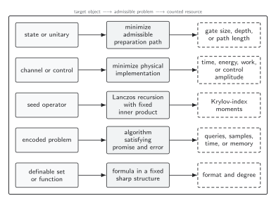
A complexity value is defined only after the target object selects an admissible family of paths or descriptions. Circuit length, physical control cost, Krylov spread, algorithmic resources, and sharp o-minimal format or degree answer different questions. The diagram is schematic and not to scale.

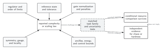
Reference sensitivity, gate nonuniqueness, regulator dependence, symmetry constraints, and unbounded controls are distinct failure modes. A link from complexity growth to chaos or computational hardness requires separate evidence after those controls. The diagram is schematic.

References

• Deffner, Sebastian, and Steve Campbell. “Quantum Speed Limits: From Heisenberg’s Uncertainty Principle to Optimal Quantum Control.” Journal of Physics A: Mathematical and Theoretical 50 (2017): 453001. DOI. Open PDF.
• Mandelstam, Leonid, and Igor Tamm. “The Uncertainty Relation Between Energy and Time in Non-relativistic Quantum Mechanics.” Journal of Physics (USSR) 9 (1945): 249–254. English translation.