Entanglement in Open and Monitored Field Dynamics

One Lindblad equation can describe many different ways of observing an environment. Those instruments agree on the state obtained after the record is discarded, but they need not agree on a nonlinear quantity evaluated along conditioned trajectories. This page makes that distinction concrete twice: first with an exactly solvable Bell pair, then with a reproducible Gaussian scalar-chain calculation in which changing only the homodyne phase changes the retained-record entanglement while leaving the unconditional evolution fixed.

Required background. Causal quantum channels supplies localized completely positive dynamics and selective versus nonselective record handling.

Helpful background. Entanglement growth supplies the closed-unitary baseline. Lindblad field dynamics owns the physical derivation, approximation domain, and continuum questions for open-QFT generators.

Unconditional state and retained record

For a finite-dimensional system, or a finite-mode regulator on which the required operators are well defined, a time-homogeneous Markovian state can obey

$$\frac{d\rho}{dt} =-i[H,\rho]+\mathcal D[L]\rho, \qquad \mathcal D[L]\rho =L\rho L^\dagger-\frac12\{L^\dagger L,\rho\}.$$

The unconditional state $\rho(t)$ predicts experiments in which the environmental record is unavailable or intentionally ignored. A unit-efficiency homodyne detector instead assigns the normalized conditioned state $\rho_c(t)$. With efficiency $\eta$, local-oscillator phase $\theta$, and $dW_t^2=dt$, one common convention is

$$d\rho_c= \left[-i[H,\rho_c]+\mathcal D[L]\rho_c\right]dt +\sqrt{\eta}\, \mathcal H[e^{-i\theta}L]\rho_c\,dW_t,$$

where

$$\mathcal H[C]\rho =C\rho+\rho C^\dagger -\operatorname{tr}\!\left[(C+C^\dagger)\rho\right]\rho.$$

The measured increment is

$$dY_\theta =\sqrt{\eta}\, \left\langle e^{-i\theta}L+e^{i\theta}L^\dagger\right\rangle_c dt +dW_t.$$

Averaging normalized trajectories with their physical probabilities recovers the unconditional state,

$$\rho(t)=\mathbb E[\rho_c(t)].$$

For the fixed Hermitian phase convention of $L$ used here, changing the local oscillator’s phase relative to $L$ changes the physical instrument. Different relative phases reveal different quadratures of one output field while unraveling the same master equation. Linear expectation values agree after record averaging; nonlinear trajectory quantities generally do not Piñol et al. 2024, Abstract and pp. L032057-1–2. That dependence does not make an unknown unraveling identifiable from the unconditional state alone: Gaona-Reyes, Altamura, and Bassi 2025, Abstract show that the relevant nonlinear averages are not operationally available without prior knowledge of the measurement scheme.

Lindblad 1976, Theorem 2 and Eqs. (4.2)–(4.3), pp. 126–127 characterizes bounded generators on $\mathcal B(\mathcal H)$; those hypotheses do not by themselves justify a pointlike unbounded field channel. For a continuum field, $H$ and $L$ may instead be unbounded operator-valued distributions. Smearing, domains, ultraviolet scaling, and the approximation producing Markovianity remain part of the physical problem. The calculation below is deliberately a fixed finite-mode regulator.

Exact Bell-state dephasing benchmark

Begin with

$$|\Phi^+\rangle =\frac{|00\rangle+|11\rangle}{\sqrt2}$$

and local phase-flip noise on $A$ with $L=\sqrt\gamma\,Z_A$. The unconditional equation is

$$\dot\rho=\gamma(Z_A\rho Z_A-\rho),$$

with exact solution

$$\rho(t)=\frac12\left[ |00\rangle\langle00|+|11\rangle\langle11| +e^{-2\gamma t} \bigl(|00\rangle\langle11|+|11\rangle\langle00|\bigr) \right].$$

The partial transpose has one negative eigenvalue $-e^{-2\gamma t}/2$. With natural logarithms,

$$\mathcal N(t)=\frac12e^{-2\gamma t}, \qquad E_{\mathcal N}(t)=\log\!\left(1+e^{-2\gamma t}\right).$$

Now retain a Poisson record of the local $Z_A$ jumps. Every trajectory is either $|\Phi^+\rangle$ or $|\Phi^-\rangle$, according to the known jump parity. The two states differ by a known local unitary, so every trajectory keeps $\mathcal N=1/2$ and $E_{\mathcal N}=\log2$. Forgetting that parity produces the decaying unconditional state.

Meanwhile $\rho_A=\mathbf1/2$ and $S(\rho_A)=\log2$ in both descriptions at every time. The unconditional state nevertheless approaches the separable mixture

$$\frac12|00\rangle\langle00| +\frac12|11\rangle\langle11|.$$

Subsystem entropy has therefore remained constant while mixed-state entanglement vanished. This exact example isolates three lessons before any field calculation: the record matters, averaging and applying a nonlinear diagnostic do not commute, and $S(\rho_A)$ is not an entanglement measure when the global state is mixed.

A cut Gaussian chain under local monitoring

The field benchmark uses dimensionless canonical quadratures

$$\mathbf R=(Q_1,\ldots,Q_N,P_1,\ldots,P_N)^{\mathsf T}, \qquad [R_\alpha,R_\beta]=i\Omega_{\alpha\beta}, \qquad \Omega= \begin{pmatrix} \mathbf0&\mathbf1\\ -\mathbf1&\mathbf0 \end{pmatrix}.$$

They may be obtained from unit-mass coordinates by $Q_j=\sqrt J\,q_j$ and $P_j=p_j/\sqrt J$. In these variables,

$$\frac{H_0}{J} =\frac12\sum_{j=1}^{N} \left[P_j^2+\mu^2Q_j^2\right] +\frac12\sum_{j=1}^{N-1}(Q_{j+1}-Q_j)^2, \qquad \mu=\frac mJ=0.7.$$

The primary chain has $N=16$ and open boundaries. It begins in the exact ground state of the uncut Hamiltonian. At dimensionless time $\tau=Jt=0$, remove the spring between sites $8$ and $9$, so

$$H_{\rm cut}=H_A+H_B, \qquad A=\{1,\ldots,8\}, \qquad B=\{9,\ldots,16\}.$$

Then monitor the last site of $A$ with

$$L=\sqrt\kappa\,Q_8, \qquad \lambda=\frac{\kappa}{J}.$$

The central cut is a scientific control, not a decorative quench. After it, both the Hamiltonian and the monitoring channel are local with respect to the full left-half–right-half bipartition. They cannot hide a new interaction across the cut.

Let $K_0$ be the dimensionless stiffness matrix before the cut. In the grouped $Q$-then-$P$ ordering, the initial covariance is

$$V_0=\frac12 \begin{pmatrix} K_0^{-1/2}&0\\ 0&K_0^{1/2} \end{pmatrix},$$

whose full-system symplectic eigenvalues are all $1/2$. The benchmark freezes

$$\lambda\in\{0,0.02,0.05,0.10,0.20,0.40\}, \qquad 0\leq\tau\leq6.$$

No trajectory is postselected.

Conditional covariance and trajectory entanglement

Write

$$V_{\alpha\beta} =\frac12\left\langle \{\Delta R_\alpha,\Delta R_\beta\} \right\rangle_c,$$

let $\mathbf e$ select $Q_8$, set $\mathbf u=\Omega\mathbf e$, and define the post-cut drift

$$\mathsf A=\Omega \begin{pmatrix} K_{\rm cut}&0\\ 0&\mathbf1 \end{pmatrix}.$$

The unconditional covariance obeys

$$\frac{dV_{\rm u}}{d\tau} =\mathsf A V_{\rm u} +V_{\rm u}\mathsf A^{\mathsf T} +D, \qquad D=\lambda\,\mathbf u\mathbf u^{\mathsf T}.$$

The Hermitian channel therefore adds momentum diffusion at the monitored site. For a retained homodyne record, the conditional first moments and centered covariance obey

$$d\overline{\mathbf R} =\mathsf A\overline{\mathbf R}\,d\tau +\mathbf b_\theta\,dW_\tau,$$ $$\frac{dV_\theta}{d\tau} =\mathsf A V_\theta +V_\theta\mathsf A^{\mathsf T} +D-\mathbf b_\theta\mathbf b_\theta^{\mathsf T},$$

with

$$\mathbf b_\theta =\sqrt{\eta\lambda} \left( 2\cos\theta\,V_\theta\mathbf e +\sin\theta\,\mathbf u \right).$$

The covariance equation is a deterministic Riccati equation, even though the record and first moments remain stochastic. That is why every trajectory in this particular linear-Gaussian protocol has the same covariance and the same displacement-invariant entanglement, but not the same state. Genoni, Lami, and Serafini 2016, § 5, Eqs. (65)–(70) derive the general conditional Gaussian equations in a covariance normalization that differs from the vacuum-$1/2$ convention used here; Minoguchi, Rabl, and Buchhold 2022, § 3.1, Eqs. (19)–(23), pp. 10–12 specialize this Kalman/Riccati structure to monitored free bosons.

The classical covariance $\Sigma_\theta$ of the conditioned first moments satisfies

$$\frac{d\Sigma_\theta}{d\tau} =\mathsf A\Sigma_\theta +\Sigma_\theta\mathsf A^{\mathsf T} +\mathbf b_\theta\mathbf b_\theta^{\mathsf T}, \qquad \Sigma_\theta(0)=0.$$

Adding the last two equations gives the exact record-average identity

$$V_{\rm u}=V_\theta+\Sigma_\theta.$$

Thus averaging only the centered conditional covariances would miss the fluctuations of the trajectory means.

To measure entanglement, reverse every momentum in $B$ and compute the symplectic eigenvalues $\widetilde\nu_k$ of the partially transposed covariance. In the vacuum-$1/2$ convention,

$$E_{\mathcal N}(V) =\sum_k \max\!\left\{0,-\log(2\widetilde\nu_k)\right\}.$$

Positive $E_{\mathcal N}$ certifies negative-partial-transpose entanglement. Because this is an $8$-mode by $8$-mode partition, $E_{\mathcal N}=0$ would establish only positivity under partial transpose, not general separability. The trace-norm definition follows Vidal and Werner 2002, Eqs. (1)–(2), pp. 032314-1–2; this page converts their base-two logarithm to the natural-log convention used throughout the calculation.

One master equation, two unravelings

For $\theta=0$, the record contains information about $Q_8$ and

$$\frac{dV_{\theta=0}}{d\tau} =\mathsf A V_{\theta=0}+V_{\theta=0}\mathsf A^{\mathsf T} +D -4\eta\lambda V_{\theta=0}\mathbf e\mathbf e^{\mathsf T}V_{\theta=0}.$$

The last term is the conditioning update: acquiring information narrows part of the covariance while the channel supplies backaction.

For $\theta=\pi/2$, the measured output contains no system-observable signal because $\cos\theta=0$. It is a no-knowledge record. At perfect efficiency,

$$\mathbf b_{\pi/2}\mathbf b_{\pi/2}^{\mathsf T}=D,$$

so diffusion cancels in the centered conditional covariance:

$$\frac{dV_{\pi/2}}{d\tau} =\mathsf A V_{\pi/2} +V_{\pi/2}\mathsf A^{\mathsf T}.$$

The state is not following deterministic closed dynamics. Its means still receive a known stochastic momentum displacement. In Stratonovich language, the record drives a stochastic Hamiltonian proportional to $Q_8$ Szigeti et al. 2014, Eqs. (5)–(7), pp. 020407-2–3. Because both that drive and $H_{\rm cut}$ are local across $A:B$, every retained-record realization is related by local unitaries. Its full-half-chain logarithmic negativity is therefore exactly constant.

The figure compares the consequences. Inspect first the separation among the four curves at $\lambda=0.10$, then whether the rate sweep preserves the same ordering.

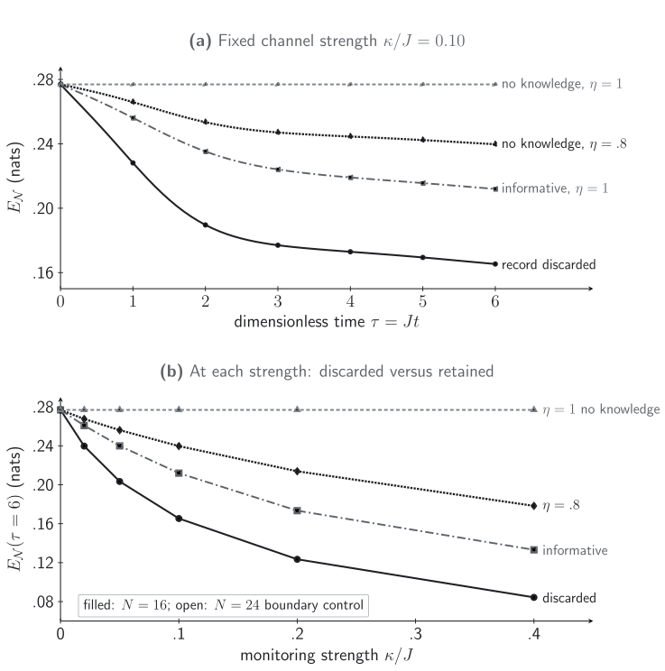
Discarded versus retained records at a fixed finite regulator. Panel (a) uses $N=16$, $m/J=0.7$, $\kappa/J=0.10$, the bond cut between sites $8$ and $9$, the full half-chain partition, and $L=\sqrt\kappa\,Q_8$. At $\tau=6$, record-discarded evolution has $E_{\mathcal N}=0.16535$, the informative $\theta=0$ record has $0.21196$, perfect-efficiency no-knowledge monitoring at $\theta=\pi/2$ retains the exact initial value $0.27691$, and the $\eta=0.8$ no-knowledge record has $0.23973$. Panel (b) sweeps the six frozen strengths at $\tau=6$; at each strength the discarded and retained evolutions share one unconditional generator. Open $N=24$ markers are the finite-boundary control. No trajectory is postselected. Curves are deterministic covariance results, not trajectory-sampling means or confidence intervals. The image is quantitative only for the declared chain, time window, partition, and instrument; it does not show feedback-based decoherence cancellation, a measurement-induced phase transition, a continuum limit, universal scaling, or an interacting-QFT result.

The unconditional curve does not depend on which homodyne phase would have been measured. At $\lambda=0.10$ and $\tau=6$, the same unconditional state has $E_{\mathcal N}=0.1653458$, whereas the informative and no-knowledge trajectory values are $0.2119594$ and $0.2769088$. The master equation fixes the first number. It does not, by itself, fix either nonlinear trajectory number.

Unraveling, efficiency, and regulator controls

At efficiency $\eta<1$, the no-knowledge centered covariance retains the unobserved diffusion:

$$\frac{dV_{\pi/2,\eta}}{d\tau} =\mathsf A V_{\pi/2,\eta} +V_{\pi/2,\eta}\mathsf A^{\mathsf T} +(1-\eta)D.$$

Consequently this benchmark has the exact downgrade control

$$V_{\pi/2,\eta=0.8}(\lambda,\tau) =V_{\rm u}(0.2\lambda,\tau).$$

At $\lambda=0.10$ and $\tau=6$, its logarithmic negativity is $0.2397349$, below the ideal record but above the discarded-record value. At $\lambda=0.40$, the four values are $0.0843231$ unconditional, $0.1331650$ informative, $0.1783290$ inefficient no-knowledge, and $0.2769088$ ideal no-knowledge.

The numerical calculation uses fixed-step RK4 with $\Delta\tau=0.0025$ and samples every $0.1$. Halving the step changes any displayed logarithmic negativity by at most $1.85\times10^{-11}$. Repeating the full grid at $N=24$, with the central bond shifted to sites $12$–$13$ and the monitored site shifted to $12$, changes it by at most $2.75\times10^{-5}$. The largest record-average covariance residual is $2.11\times10^{-14}$ in Frobenius norm. The perfect no-knowledge covariance differs from exact Hamiltonian propagation by at most $7.38\times10^{-11}$.

These are deterministic integration and finite-boundary controls, not statistical error bars. The benchmark also checks covariance symmetry, $V+i\Omega/2\geq0$, pure-state symplectic normalization under efficient conditioning, the $\kappa=0$ unitary control, and the exact $(1-\eta)D$ identity. It does not take $N\to\infty$, restore a physical lattice spacing, smear the monitored field, or control indefinite environmental heating.

The exact invariance has a deliberately narrow hypothesis set. Restoring the central spring, moving the diagnostic away from the full $A:B$ split, changing $\theta$ away from $\pi/2$, lowering $\eta$, adding an unmonitored channel, using a non-Hermitian jump operator, or discarding the record removes at least one step of the local-unitary proof.

Monitored many-body dynamics

Hybrid unitary–measurement circuits provide broader models in which gates create trajectory entanglement and measurements suppress it. At low measurement rate, typical conditioned trajectories can retain volume-law entanglement; at high rate, they can have area-law entanglement. Finite-size scaling can identify a transition in specified circuit and spin-chain classes Li, Chen, and Fisher 2018, §§ II–IV; Skinner, Ruhman, and Nahum 2019, §§ II–IV.

That literature does not turn the finite Gaussian sweep above into a transition:

• the transition concerns a specified ensemble of conditioned trajectories;
• measurement basis, location, symmetry, efficiency, and unitary ensemble can change the critical data;
• the exactly solvable percolation mapping applies to a zeroth-Rényi toy limit, not automatically to von Neumann entropy;
• the unconditional mixed state solves a different entanglement problem;
• postselection probability and trajectory-sampling cost are operational resources;
• a continuum monitored field needs locality, energy, smearing, and cutoff convergence beyond finite-size circuit collapse.

Hardware estimators must also be named precisely. Kamakari et al. 2025, Abstract, Eq. (1), and Figs. 3–4 use a scalable cross-entropy-benchmarking proxy on superconducting processors. That is evidence for the studied circuits and estimator, not a direct large-system measurement of von Neumann trajectory entropy or a continuum universality theorem.

Reproducibility and stop rule

Download the quantitative SVG, complete covariance diagnostics and controls, compact plot-view CSV, and JSON protocol, equations, assertions, and claim boundary. The compact view is generated from the complete calculation and adds no fitted values.

What survives every declared control is specific: for this finite gapped Gaussian chain, exact central cut, local Hermitian channel, full half-chain partition, retained record, and perfect efficiency, changing the homodyne phase leaves the unconditional Lindblad state fixed but changes conditioned logarithmic negativity. The no-knowledge phase converts the observed backaction into a known local stochastic displacement and preserves each trajectory’s initial entanglement. The result does not establish decoherence cancellation without feedback, a measurement-induced transition, continuum existence, universal scaling, or an interacting-QFT law.

The chapter orientation map separates monitored from closed-unitary dynamics. Its failure controls require the record and nonlinear estimator to be varied, while the diagnostic comparison keeps trajectory entanglement distinct from the unconditional mixed state.

Common pitfalls

Ignoring the relative homodyne phase. Once the phase convention for $L$ is fixed, the local oscillator selects which output quadrature is measured and therefore which record-conditioned instrument is realized. A simultaneous rephasing of $L$ and the reference is a convention; changing their relative phase is not. Only the record-discarded generator is phase independent here.

Saying that no-knowledge monitoring cancels decoherence. Without feedback, discarded records still reproduce the diffusive master equation. At $\eta=1$, only the centered conditional covariance loses its diffusion term; known stochastic local displacements remain.

Averaging in the wrong order. The unconditional covariance is $V_c+\operatorname{Cov}(\overline{\mathbf R})$, not merely the average centered covariance. Likewise, $E_{\mathcal N}(\mathbb E[\rho_c])$ need not equal $\mathbb E[E_{\mathcal N}(\rho_c)]$.

Treating zero logarithmic negativity as a separability theorem. Positive logarithmic negativity certifies NPT entanglement. For this multimode split, zero detects no NPT entanglement but does not exclude every PPT-entangled Gaussian state.

Calling a finite rate sweep a phase transition. A transition claim requires a thermodynamic sequence, scaling observable, fit-window stability, trajectory convergence, and a specified universality class. This calculation supplies none of those limits.

Exercises

Derive the unconditional Bell-state dephasing solution and its logarithmic negativity.

Solution

The diagonal matrix elements are fixed. Since $Z_A|00\rangle=|00\rangle$ and $Z_A|11\rangle=-|11\rangle$, the coherence obeys

$$\dot\rho_{00,11}=-2\gamma\rho_{00,11},$$

so $\rho_{00,11}=e^{-2\gamma t}/2$. Partial transposition moves this coherence to the $|01\rangle,|10\rangle$ block, whose eigenvalues are $\pm e^{-2\gamma t}/2$. Hence

$$\|\rho^{T_A}\|_1=1+e^{-2\gamma t}, \qquad E_{\mathcal N}=\log(1+e^{-2\gamma t}).$$

Insert $\theta=\pi/2$ into the Gaussian innovation vector. Why does perfect efficiency remove diffusion from the centered conditional covariance but not from the unconditional state?

Solution

At $\theta=\pi/2$,

$$\mathbf b_{\pi/2} =\sqrt{\eta\lambda}\,\mathbf u, \qquad \mathbf b_{\pi/2}\mathbf b_{\pi/2}^{\mathsf T} =\eta D.$$

Therefore the conditional covariance contains $(1-\eta)D$ and has no diffusion at $\eta=1$. At general efficiency the trajectory means still receive $\sqrt{\eta\lambda}\,\mathbf u\,dW_\tau$; at $\eta=1$ this becomes $\sqrt\lambda\,\mathbf u\,dW_\tau$. When the no-knowledge record is discarded, their covariance is added back:

$$V_{\rm u}=V_{\pi/2}+\Sigma_{\pi/2}.$$

The unconditional equation consequently retains the full $D$.

Prove the record-average covariance identity by adding the equations for $V_\theta$ and $\Sigma_\theta$.

Solution

The information terms cancel:

$$\frac d{d\tau}(V_\theta+\Sigma_\theta) =\mathsf A(V_\theta+\Sigma_\theta) +(V_\theta+\Sigma_\theta)\mathsf A^{\mathsf T} +D.$$

Because $V_\theta(0)+\Sigma_\theta(0)=V_0$, uniqueness of the linear covariance equation gives

$$V_\theta+\Sigma_\theta=V_{\rm u}.$$

This is the law of total covariance in Gaussian-filter form.

At no-knowledge phase and efficiency $\eta=0.8$, show that the conditional covariance at strength $\lambda$ equals the unconditional covariance at strength $0.2\lambda$.

Solution

The no-knowledge Riccati subtraction leaves

$$D-\eta D=(1-\eta)D=0.2\lambda\,\mathbf u\mathbf u^{\mathsf T}.$$

The drift and initial covariance are otherwise identical to the unconditional problem. The two matrix differential equations therefore have the same unique solution. This equality concerns centered covariances and displacement-invariant diagnostics; the records and conditioned means are not the same stochastic objects.

Which step of the constant-entanglement proof fails if the central spring is restored? Which step fails if the record is discarded?

Solution

With the spring restored, $H$ no longer decomposes as $H_A+H_B$. Even a perfect no-knowledge trajectory then includes a cross-cut unitary, so local-unitary invariance cannot keep the $A:B$ entanglement constant.

If the record is discarded, the random local displacements are unknown and must be averaged. A mixture of locally related entangled states can have less entanglement than each member, as the Bell benchmark demonstrates. The unconditional covariance receives the full diffusion $D$, so its logarithmic negativity need not remain constant.

References

• Gaona-Reyes, J. L., D. G. A. Altamura, and A. Bassi. “Theoretical Limits of Protocols for Distinguishing Different Unravelings.” Physical Review Research 7 (2025): 043295. DOI.
• Genoni, Marco G., Ludovico Lami, and Alessio Serafini. “Conditional and Unconditional Gaussian Quantum Dynamics.” Contemporary Physics 57 (2016): 331–349. DOI. Open PDF.
• Kamakari, Hirsh, Jiace Sun, Yaodong Li, Jonathan J. Thio, Tanvi P. Gujarati, Matthew P. A. Fisher, Mario Motta, and Austin J. Minnich. “Experimental Demonstration of Scalable Cross-Entropy Benchmarking to Detect Measurement-Induced Phase Transitions on a Superconducting Quantum Processor.” Physical Review Letters 134 (2025): 120401. DOI.
• Li, Yaodong, Xiao Chen, and Matthew P. A. Fisher. “Quantum Zeno Effect and the Many-Body Entanglement Transition.” Physical Review B 98 (2018): 205136. DOI.
• Lindblad, Göran. “On the Generators of Quantum Dynamical Semigroups.” Communications in Mathematical Physics 48 (1976): 119–130. DOI.
• Minoguchi, Yuri, Peter Rabl, and Michael Buchhold. “Continuous Gaussian Measurements of the Free Boson CFT: A Model for Exactly Solvable and Detectable Measurement-Induced Dynamics.” SciPost Physics 12 (2022): 009. DOI.
• Piñol, Eloy, Th. K. Mavrogordatos, Dustin Keys, Romain Veyron, Piotr Sierant, Miguel Angel García-March, Samuele Grandi, Morgan W. Mitchell, Jan Wehr, and Maciej Lewenstein. “Telling Different Unravelings Apart via Nonlinear Quantum-Trajectory Averages.” Physical Review Research 6 (2024): L032057. DOI.
• Skinner, Brian, Jonathan Ruhman, and Adam Nahum. “Measurement-Induced Phase Transitions in the Dynamics of Entanglement.” Physical Review X 9 (2019): 031009. DOI.
• Szigeti, Stuart S., André R. R. Carvalho, James G. Morley, and Michael R. Hush. “Ignorance Is Bliss: General and Robust Cancellation of Decoherence via No-Knowledge Quantum Feedback.” Physical Review Letters 113 (2014): 020407. DOI.
• Vidal, Guifré, and Reinhard F. Werner. “A Computable Measure of Entanglement.” Physical Review A 65 (2002): 032314. DOI.