Petz, Rotated, and Universal Recovery Maps

Petz recovery is the reference-weighted reverse of a quantum channel. It exactly reverses every state pair that saturates relative-entropy data processing. Modularly rotated Petz maps insert reference-state modular flow before and after that reverse, and a particular weighted average of the rotations gives one explicit map with a fidelity guarantee for every support-compatible input state. “Universal” means independent of the state being recovered once the reference state and forward channel are fixed; it does not mean independent of those data, spatially local, energy bounded, or regulator independent.

Required background. Use Recovery Maps and Approximate Markovianity for the recovery task and fidelity guarantee. Helpful background. Araki Relative Entropy and Regulated Limits supplies the support and modular setting used below.

The chapter’s task-comparison table places exact and approximate recovery beside their required algebra, reference state, channel, norm, and regulator data.

The Petz transpose map on a fixed support

Work first with finite-dimensional matrix algebras in the Schrödinger picture. Here $\mathcal T(\mathcal H)$ denotes the trace-class operators on $\mathcal H$. Let

$$\mathcal N:\mathcal T(\mathcal H_A)\longrightarrow \mathcal T(\mathcal H_B)$$

be a completely positive trace-preserving channel, let $\mathcal N^\dagger$ be its adjoint—defined by $\operatorname{Tr}[Y\mathcal N(X)]=\operatorname{Tr}[\mathcal N^\dagger(Y)X]$—and fix a positive reference state $\sigma$ on $A$. Write

$$\tau=\mathcal N(\sigma),\qquad P_\sigma=\operatorname{supp}\sigma,\qquad P_\tau=\operatorname{supp}\tau.$$

The support of a positive operator is the span of its eigenvectors with nonzero eigenvalues. All negative powers below are Moore–Penrose powers: they invert the strictly positive spectrum and vanish on the kernel. The Petz map is

$$\mathcal P_{\sigma,\mathcal N}(X) =\sigma^{1/2}\, \mathcal N^\dagger\!\left( \tau^{-1/2}X\tau^{-1/2} \right)\sigma^{1/2}.$$

This formula is a noncommutative version of Bayes inversion: $\sigma$ supplies the prior, $\tau$ is the prior after the forward channel, and $\mathcal N^\dagger$ pulls an output operator back to the input. The ordering of the square roots is essential because the factors need not commute.

The map is completely positive and preserves trace on the supported input algebra. Indeed,

$$\begin{aligned} \operatorname{Tr}\mathcal P_{\sigma,\mathcal N}(X) &=\operatorname{Tr}\!\left[ \tau\,\tau^{-1/2}X\tau^{-1/2} \right]\\ &=\operatorname{Tr}(P_\tau X), \end{aligned}$$

so $\operatorname{Tr}\mathcal P(X)=\operatorname{Tr}X$ whenever $X=P_\tau XP_\tau$. To obtain a channel on all of $\mathcal T(\mathcal H_B)$, choose any state $\omega_0$ supported in $P_\sigma$ and extend it by

$$\widehat{\mathcal P}(X) =\mathcal P(P_\tau XP_\tau) +\operatorname{Tr}[(I_B-P_\tau)X]\,\omega_0.$$

The extension is completely positive and trace preserving. Its arbitrary action outside $P_\tau$ cannot affect a state produced from a support-compatible input by $\mathcal N$.

The exact theorem is now clean. If $\operatorname{supp}\rho\subseteq\operatorname{supp}\sigma$ and

$$D(\rho\Vert\sigma) =D\!\left(\mathcal N(\rho)\Vert\mathcal N(\sigma)\right)<\infty,$$

then

$$\mathcal P_{\sigma,\mathcal N}(\mathcal N(\rho))=\rho, \qquad \mathcal P_{\sigma,\mathcal N}(\mathcal N(\sigma))=\sigma.$$

Conversely, any channel that recovers both $\rho$ and $\sigma$ forces equality by applying data processing first to $\mathcal N$ and then to the recovery channel. Petz’s sufficiency theorem proves the nontrivial equality-to-recovery direction in von Neumann algebras Petz 1986, Theorems 4–5, pp. 126–129. Faithfulness is a convenient way to avoid writing support projectors; it is not a license to ignore a kernel.

The structure diagram locates this construction on the channels-and-recovery branch. Inspect how correlation data and resource constraints select that branch; after it is selected, changing the reference state or adjoint changes the recovery problem even if the forward input and output spaces have the same names.

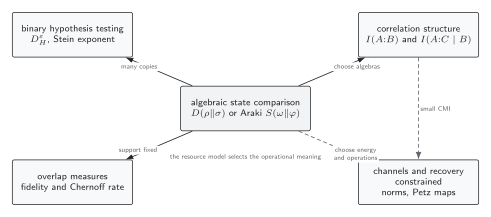
Relative entropy alone does not select an operational task. Correlation and resource data select the recovery branch; Petz, rotated, and universal maps then additionally require a declared channel, reference, support, and regulator. Schematic.

Modular rotations and the universal average

For a positive state $\omega$, define modular conjugation on its support by

$$\alpha_t^\omega(X)=\omega^{it}X\omega^{-it}.$$

Our sign convention for a rotated Petz map is

$$\mathcal R_{\sigma,\mathcal N}^{\,t} =\alpha_t^\sigma\circ \mathcal P_{\sigma,\mathcal N}\circ \alpha_{-t}^{\tau}.$$

Equivalently,

$$\mathcal R_{\sigma,\mathcal N}^{\,t}(X) =\sigma^{1/2+it} \mathcal N^\dagger\!\left( \tau^{-1/2-it}X\tau^{-1/2+it} \right) \sigma^{1/2-it}.$$

Some sources replace $t$ by $-t$. Nothing below changes because the averaging density is even. Each fixed-$t$ map is completely positive and trace preserving on the same supported input algebra as the Petz map, and $t=0$ gives $\mathcal P$.

Define

$$\beta_0(t) =\frac{\pi}{2[\cosh(\pi t)+1]} =\frac{\pi}{4}\operatorname{sech}^2\!\left(\frac{\pi t}{2}\right), \qquad \int_{-\infty}^{\infty}\beta_0(t)\,\mathrm dt=1,$$

and form the twirled map

$$\overline{\mathcal R}_{\sigma,\mathcal N} =\int_{-\infty}^{\infty} \beta_0(t)\, \mathcal R_{\sigma,\mathcal N}^{\,t/2}\,\mathrm dt.$$

For the root fidelity

$$F(\rho,\omega)= \left\lVert\sqrt\rho\sqrt\omega\right\rVert_1$$

and natural logarithms, the universal recovery theorem states

$$\begin{aligned} \Delta_{\sigma,\mathcal N}(\rho) &\equiv D(\rho\Vert\sigma) -D\!\left(\mathcal N(\rho)\Vert\mathcal N(\sigma)\right)\\ &\geq-2\log F\!\left( \rho, (\overline{\mathcal R}_{\sigma,\mathcal N}\circ\mathcal N)(\rho) \right). \end{aligned}$$

The same $\overline{\mathcal R}_{\sigma,\mathcal N}$ works for every $\rho$ supported in $\sigma$, depends only on $\sigma$ and $\mathcal N$, and exactly recovers $\sigma$. The stronger form averages $-\log F$ over the individual rotations before passing to the averaged channel Junge et al. 2018, Theorem 2.1 and Remark 2.2. If $\Delta=0$, every rotation recovers the equality pair, not merely the average.

The three constructions answer different questions:

Construction	Extra choice	Exact equality	Generic approximate guarantee
Petz	none after $\sigma$ and $\mathcal N$	recovers every equality pair	no general Umegaki-loss fidelity bound of the displayed universal form
Rotated Petz	one modular time $t$	every $t$ recovers an equality pair	a suitable rotation can improve recovery, but a fixed unaveraged $t$ is not the universal theorem
Universal average	the fixed density $\beta_0$	recovers $\sigma$ and every equality pair	one explicit state-independent map obeys the displayed bound for all support-compatible $\rho$

Here “rotation” is modular evolution generated by $\log\sigma$ and $\log\tau$, not a spatial rotation. If a physical symmetry intertwines $\mathcal N$ and leaves $\sigma$ invariant, then the Petz formula and its twirl inherit that covariance. Without those hypotheses, modular covariance does not imply Lorentz covariance, causal localization, or symmetry-respecting laboratory control.

A finite free-fermion field reduction

A regulated free fermion supplies a useful QFT test because a Gaussian state is determined by finitely many two-point functions. For Majorana operators $\gamma_j$ with $\{\gamma_j,\gamma_k\}=2\delta_{jk}$, use the real antisymmetric covariance matrix

$$G_{jk}=\frac{i}{2}\operatorname{Tr}\!\left(\rho[\gamma_j,\gamma_k]\right).$$

A fermionic Gaussian channel acts as $G\mapsto BGB^{\mathsf T}+A$. If the reference and channel are Gaussian, then the Petz map is Gaussian too, with

$$\begin{aligned} B_{\mathcal P} &=\sqrt{I+G_\sigma^2}\,B^{\mathsf T} \left(\sqrt{I+G_\tau^2}\right)^{-1},\\ A_{\mathcal P} &=G_\sigma-B_{\mathcal P}G_\tau B_{\mathcal P}^{\mathsf T}. \end{aligned}$$

Modular conjugation is a Gaussian unitary, so every rotated Petz map is again Gaussian. These covariance formulas, their rotated counterparts, and the limiting treatment required at singular matrices are derived by Swingle and Wang 2019, Eqs. (7)–(8) and Appendix C. The bosonic analogue is also a Gaussian channel Lami, Das, and Wilde 2018, Theorem 1 and Corollary 2. A convex average of Gaussian channels, however, need not itself be a single Gaussian channel; the twirl should be evaluated as the stated mixture unless an additional closure argument applies.

The reproducible recovery benchmark uses the Gibbs state of a five-site open spinless free-fermion chain. In this subsection, $A$, $B$, and $C$ label spatial regions rather than the generic channel input and output spaces used above. The Hamiltonian is

$$H=\sum_{i,j}h_{ij}c_i^\dagger c_j, \qquad h_{ii}=\mu+(-1)^i m, \qquad h_{i,i+1}=h_{i+1,i}=-\kappa,$$

with $\kappa=1$, $m=0.7$, $\mu=0.15$, and inverse temperature $\beta=1.4$. The contiguous partition is $A=\{0\}$, $B=\{1,2,3\}$, and $C=\{4\}$. For the local channel $\mathcal N=\operatorname{Tr}_C:BC\to B$, take $\sigma=\rho_{BC}$ and $\tau=\rho_B$; the recovered global state is

$$\widetilde\rho_{ABC} =(\operatorname{id}_A\otimes\mathcal R_{B\to BC})(\rho_{AB}).$$

Thus the recovery map depends on $\rho_{BC}$ but not on the remote system $A$. The record freezes the occupation-number basis, Hamiltonian and state parameters, region ordering, modular-time quadrature, spectral inverse policy, root-fidelity convention, and numerical precision.

At this regulator, the conditional mutual information is

$$I(A{:}C\mid B)=3.645078306\times10^{-4}\ \text{nats},$$

so the theorem alone guarantees $F\geq0.9998177627$. Direct evaluation gives:

Recovery applied to $\rho_{AB}$	Root fidelity	$-2\log F$ (nats)	Trace-norm error
Ordinary Petz	$0.9999963358$	$7.3284\times10^{-6}$	$0.00494216$
Equal mixture at theorem variables $t=\pm1$ (modular parameters $t/2=\pm0.5$)	$0.9999831052$	$3.37898\times10^{-5}$	$0.0106291$
Universal $\beta_0$ twirl, 64 nodes	$0.9999988099$	$2.38012\times10^{-6}$	$0.00278284$
Petz acting only on the edge site of $B$	$0.9974519102$	$5.10268\times10^{-3}$	$0.132236$

The symmetric two-point mixture is a diagnostic, not the universal average. In this example the bare Petz map happens to perform extremely well, but no general bare-Petz version of the displayed Umegaki-loss bound is being asserted. The 16-, 32-, and 64-node twirls have a root-fidelity envelope of $9.41\times10^{-8}$; this is a deterministic quadrature-resolution diagnostic, not a statistical error bar or a rigorous all-orders integration bound. The full-$B$ universal result satisfies $-2\log F<I(A{:}C\mid B)$ by more than two orders of magnitude. The deliberately edge-only channel solves a smaller recovery problem, so its poorer fidelity does not contradict the theorem.

The calculation is reproducible in five steps:

1. Diagonalize the $5\times5$ one-body Hamiltonian, build its Fermi–Dirac correlation matrix, and independently reconstruct the $2^5\times2^5$ Gibbs density matrix. Their one-body correlators agree to $7.8\times10^{-16}$ in the record.
2. Form $\rho_{ABC}$, $\rho_{AB}$, $\sigma=\rho_{BC}$, and $\tau=\rho_B$ by exact partial traces. Diagonalize $\sigma$ and $\tau$, retain their positive supports, and construct $X^{\pm1/2}$ and $X^{it}$ spectrally on those supports.
3. Apply the density-matrix formula for $\mathcal P$ and the modular conjugations for each sampled $t$. Check Hermiticity, positivity, trace, and exact recovery of $\sigma$ before comparing the target state.
4. Set $u=[1+\tanh(\pi t/2)]/2$, for which $\beta_0(t)\,\mathrm dt=\mathrm du$. At $n$ nodes, evaluate the rotations at $u_j=(j+\tfrac12)/n$ and $t_j=(2/\pi)\operatorname{artanh}(2u_j-1)$, then take their equal-weight average. This quantile midpoint rule covers the full probability interval; the 16-, 32-, and 64-node spread measures refinement, not a rigorous quadrature remainder.
5. Report root fidelity to $\rho_{ABC}$, conditional mutual information, the theorem residual $I(A{:}C\mid B)+2\log F$, the smallest supported eigenvalue, and the inverse-square-root condition number. Repeat at 16, 32, and 64 modular quadrature nodes and require byte-for-byte regeneration of the public record.

The benchmark is a finite, bounded first application. Agreement with the recovery inequality tests the implementation; it does not prove that the recovery has a normal, local, energy-feasible continuum limit. The covariance description verifies the Gaussian structure of each unaveraged map, while the density-matrix route keeps the support convention and the non-Gaussian twirled mixture explicit.

Rank loss and modular-domain stress tests

The inverse square root makes support part of the theorem rather than a numerical nuisance. If the smallest positive eigenvalue of $\tau$ is $\lambda_{\min}^+$, then

$$\left\lVert\tau^{-1/2}\right\rVert =\frac{1}{\sqrt{\lambda_{\min}^+}}.$$

Consequently, perturbations in the small-eigenvalue sector are magnified before the outer $\sigma^{1/2}$ factors can cancel them. Exact arithmetic may remain benign while a floating-point implementation becomes unreliable. A cutoff rule must therefore report both the discarded spectral weight and the effect on recovered observables; a small trace defect alone is not a stability certificate.

The benchmark approaches rank deficiency by increasing the inverse temperature through $\beta=0.5,1,2,4,8$ while keeping the Hamiltonian, channel, partition, and basis fixed. Across that sweep, the condition number of $\rho_B$ grows from $6.19$ through $32.2$, $341$, and $3565$ to $1.11\times10^5$; at $\beta=8$, $\lVert\rho_B^{-1/2}\rVert=397.63$. Because changing $\beta$ also changes the state and its conditional mutual information, this sweep diagnoses the combined low-temperature problem rather than attributing every fidelity change to conditioning alone.

A second test at fixed $\beta=8$ isolates the numerical inverse policy. Floors at $10^{-8}$ and $10^{-6}$ times the largest eigenvalue remain below the true smallest eigenvalue and leave the calculation unchanged. A floor of $10^{-4}$ times the largest eigenvalue clamps three positive eigenvalues upward before inversion and creates a trace defect of $3.37\times10^{-5}$; it does not project those eigenspaces away. Normalizing the output before checking whether the map is a channel would divide away this defect and conceal the failure. At an exact zero eigenvalue, the correct operation is instead to reduce to the new support and define a channel extension there. Replacing $\tau^{-1/2}$ by $(\tau+\varepsilon I)^{-1/2}$ changes the map; it is a Petz map for a regularized problem only if $\sigma$ and $\tau=\mathcal N(\sigma)$ are changed consistently.

The lower diagram summarizes the corresponding continuum warning. In a sharp-region QFT, the local algebra is generally type III and no regional density matrix $\sigma$ exists. Relative modular operators and normal maps replace the displayed matrix inverses, with analytic cores and domains specified. The rigorous algebraic equality theorem belongs to Sufficiency, Conditional Expectations, and Petz Recovery. Even when an abstract recovery map exists, energy-constrained channel distances are needed before claiming finite-resource approximation.

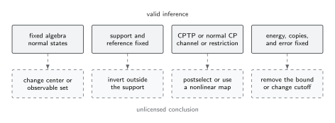
Support reduction repairs a singular finite-dimensional formula only on the declared support. It does not by itself establish a bounded modular operation, causal localization, or controlled energy cost when the field regulator is removed. Schematic.

What a defensible recovery claim reports

A reproducible claim names the Schrödinger or Heisenberg picture; the channel and adjoint pairing; $\rho$, $\sigma$, and their supports; the modular sign convention; the fidelity convention and logarithm base; the rotation or quadrature measure; the regulator and order of limits; and any locality, symmetry, or energy constraint. It separately checks recovery of the reference, positivity and trace preservation, numerical conditioning, the theorem residual, and stability under refinement.

The central comparison can then be stated precisely. Petz is the canonical reference-weighted reverse and owns exact sufficiency. Rotations explore the reference modular orbit. The $\beta_0$ average turns those rotations into one explicit map with a uniform fidelity remainder bound. None of these algebraic properties alone turns the map into an attainable local QFT protocol.

Common pitfalls

Inverting before restricting the support. A tiny eigenvalue is not the same as a zero eigenvalue. Use spectral support explicitly, report its threshold in numerical work, and treat a changed support as a changed problem.

Calling every Petz map universal. The ordinary Petz map already depends only on $\sigma$ and $\mathcal N$, but the word “universal” in the remainder theorem means that one explicit averaged map obeys the same guarantee for every compatible $\rho$.

Confusing modular and spacetime motion. The parameter $t$ generates conjugation by a density operator or modular operator. It is not physical time, a Lorentz transformation, or a local circuit depth unless an additional theorem identifies those structures.

Averaging covariance matrices instead of channels. Each rotated Gaussian channel has its own action on the state. Average the output states or channels with $\beta_0$; averaging Gaussian channel parameters generally solves a different problem.

Exercises

1. Trace preservation on the supported algebra

Prove that $\mathcal P_{\sigma,\mathcal N}$ preserves trace on $P_\tau\mathcal H_B$, and verify that $\widehat{\mathcal P}$ is a channel on the full input algebra.

Solution

For $X=P_\tau XP_\tau$, adjointness and cyclicity give

$$\begin{aligned} \operatorname{Tr}\mathcal P(X) &=\operatorname{Tr}\!\left[ \mathcal N(\sigma)\tau^{-1/2}X\tau^{-1/2} \right]\\ &=\operatorname{Tr}(P_\tau X) =\operatorname{Tr}X. \end{aligned}$$

Both terms in $\widehat{\mathcal P}$ are completely positive. For arbitrary $X$,

$$\operatorname{Tr}\widehat{\mathcal P}(X) =\operatorname{Tr}(P_\tau X) +\operatorname{Tr}[(I_B-P_\tau)X] =\operatorname{Tr}X.$$

Thus the extension is CPTP. Its measure-and-prepare term is irrelevant on the supported outputs of $\mathcal N$.

2. Why rotations disappear classically

Suppose $\sigma$, $\tau$, and every input $X$ are diagonal in the bases in which a classical channel is represented. Show that every rotated Petz map equals the ordinary Petz map.

Solution

Diagonal matrices commute, so

$$\alpha_{-t}^{\tau}(X) =\tau^{-it}X\tau^{it}=X.$$

The output of the classical Petz map is diagonal as well, hence

$$\alpha_t^\sigma(\mathcal P(X))=\mathcal P(X).$$

Therefore $\mathcal R^t=\mathcal P$ for every $t$, and the $\beta_0$ average also equals $\mathcal P$. A nontrivial modular-time dependence is a genuinely noncommutative effect.

3. From entropy loss to a fidelity target

Let $\Delta_{\sigma,\mathcal N}(\rho)\leq\delta$. Use the universal bound to find a guaranteed fidelity and a trace-distance estimate.

Solution

The theorem gives

$$-2\log F\leq\delta,$$

so

$$F\geq e^{-\delta/2}.$$

For root fidelity, Fuchs and van de Graaf 1999, Theorem 1 and Eq. (46), pp. 1222–1223 gives

$$\frac12\left\lVert \rho-(\overline{\mathcal R}\circ\mathcal N)(\rho) \right\rVert_1 \leq\sqrt{1-F^2} \leq\sqrt{1-e^{-\delta}}.$$

This estimates state error only. It contains no bound on the energy, spatial support, circuit cost, or implementation time of $\overline{\mathcal R}$.

4. An exactly cancelling but ill-conditioned inverse

Take $\mathcal N$ to be the identity channel and

$$\sigma_\varepsilon =\begin{pmatrix}1-\varepsilon&0\\0&\varepsilon\end{pmatrix}, \qquad 0<\varepsilon<\frac12.$$

Show that the Petz map is exactly the identity, but identify an intermediate operation whose norm diverges as $\varepsilon\to0^+$.

Solution

Here $\tau=\sigma_\varepsilon$ and $\mathcal N^\dagger$ is the identity, so

$$\mathcal P(X) =\sigma_\varepsilon^{1/2} \sigma_\varepsilon^{-1/2}X \sigma_\varepsilon^{-1/2} \sigma_\varepsilon^{1/2} =X.$$

The cancellation is exact for every $\varepsilon>0$. Nevertheless,

$$\left\lVert\sigma_\varepsilon^{-1/2}\right\rVert =\varepsilon^{-1/2},$$

and the inner sandwich sends $|1\rangle\!\langle1|$ to $\varepsilon^{-1}|1\rangle\!\langle1|$. Finite-precision errors in that eigenspace are therefore strongly amplified before the outer factors cancel them. At $\varepsilon=0$ the support changes and the generalized-inverse construction must be interpreted on the one-dimensional support; substituting a large finite inverse is not the same operation.

References

• Fuchs, Christopher A., and Jeroen van de Graaf. “Cryptographic Distinguishability Measures for Quantum-Mechanical States.” IEEE Transactions on Information Theory 45, no. 4 (1999): 1216–1227. DOI.
• Junge, Marius, Renato Renner, David Sutter, Mark M. Wilde, and Andreas Winter. “Universal Recovery Maps and Approximate Sufficiency of Quantum Relative Entropy.” Annales Henri Poincaré 19, no. 10 (2018): 2955–2978. DOI. Open PDF.
• Lami, Ludovico, Siddhartha Das, and Mark M. Wilde. “Approximate Reversal of Quantum Gaussian Dynamics.” Journal of Physics A: Mathematical and Theoretical 51, no. 12 (2018): 125301. DOI. Open PDF.
• Petz, Dénes. “Sufficient Subalgebras and the Relative Entropy of States of a von Neumann Algebra.” Communications in Mathematical Physics 105, no. 1 (1986): 123–131. DOI.
• Swingle, Brian, and Yixu Wang. “Recovery Map for Fermionic Gaussian Channels.” Journal of Mathematical Physics 60, no. 7 (2019): 072202. DOI. Open PDF.