Membrane, Hydrodynamic, and Coarse-Grained Entanglement Laws

In a chaotic, locally equilibrating system, the leading entropy of a large region can sometimes be obtained by minimizing an effective membrane action in spacetime. The membrane compresses complicated microscopic dynamics into a model-dependent tension $\mathcal E(v)$. It is a long-distance law for entanglement geometry—not a microscopic equation of motion, not ordinary charge hydrodynamics, and not a default replacement for the quasiparticle picture in integrable systems.

Required background. Entanglement growth after quenches supplies the entropy profiles that the effective law must reproduce.

Helpful background. Quasiparticle growth supplies a contrasting mechanism whose persistent mode occupations are normally incompatible with a single chaotic membrane tension.

Unless an index is shown explicitly, $S$ denotes von Neumann entropy $S_1=-\operatorname{tr}(\rho\ln\rho)$ in nats. Rényi entropies can have different effective tensions, so changing the entropy species changes the claim rather than merely the notation.

The one-dimensional variational law

Let $S(x,t)$ denote the coarse-grained entropy across the cut at position $x$. On the physical membrane branch, write $v_{\max}$ for the largest slope needed by the minimization. A convenient one-dimensional convention is

$$S(x,t)=\min_{|x-y|\leq v_{\max}t}\left[ S(y,0)+s_{\rm eq}t\, \mathcal E\!\left(\frac{x-y}{t}\right) \right].$$

$s_{\rm eq}$ is the equilibrium entropy density, and the argument

$$v=\frac{x-y}{t}$$

is the spatial slope of a straight membrane segment in spacetime. The formula says that the final cut can inherit initial entanglement from a different position $y$, at the cost of a membrane segment connecting $(y,0)$ to $(x,t)$. Equivalently, one may minimize over all $y$ after extending the effective tension by $\mathcal E_{\rm eff}(v)=|v|$ for $|v|\geq v_{\max}$.

For parity-symmetric homogeneous dynamics and a spatially homogeneous low-entanglement initial state, the minimum is at $v=0$. Far from physical boundaries and before saturation, a single cut then grows as

$$S(x,t)-S(x,0)=s_{\rm eq}\mathcal E(0)t.$$

More generally $v_E=\Gamma(0)=\min_v\mathcal E(v)$. In the parity-symmetric convention used here,

$$v_E=\mathcal E(0).$$

Other papers absorb factors of $s_{\rm eq}$, boundary area, or time into the tension. Always reproduce the defining action before comparing quoted values of $v_E$.

The membrane proposal, its operator-entanglement extraction, and the endpoint-speed caveat are developed by Jonay, Huse, and Nahum 2018, § II.A, Eqs. (4)–(13). In random unitary circuits, literal bond-counting minimal cuts are controlled in the large-local-dimension limit; finite local dimension brings entropy-index and fluctuation corrections. With temporal randomness in one dimension, the leading mean can have KPZ fluctuations around it Nahum et al. 2017, §§ II–V. Holographic calculations provide a distinct setting whose large-region limit takes the same membrane form Mezei 2018, §§ II–III.

The effective law is not confined to averaged circuits, but its microscopic justification remains model dependent. Zhou and Nahum 2020, abstract and §§ I–VI construct a consistent line tension for translationally invariant chaotic Floquet chains and find that generic and dual-unitary models need not share the same tension. In an exactly solvable family of generalized dual-unitary circuits, Rampp, Rather, and Claeys 2024, abstract and §§ II–IV obtain nontrivial tensions and a hierarchy with $v_E<v_B$. These examples support the membrane framework while warning against importing one model’s tension or velocity relations into another; Fisher et al. 2023, pp. 335–379 give broader context for which random-circuit conclusions are universal and which rely on tractable ensembles.

Tension constraints and their scope

For parity-symmetric homogeneous dynamics, $\mathcal E(v)$ is even. Stability of the variational problem requires the relevant branch to be convex. In the standard chaotic membrane convention, one also finds

$$\mathcal E(0)=v_E, \qquad \mathcal E(v_{\max})=v_{\max}, \qquad \mathcal E'(v_{\max})=1, \qquad \mathcal E(v)\geq |v|,$$

on the physical branch. The Legendre structure supplies the endpoint speed $v_{\max}=-\Gamma'(1)$ in this normalization. Identifying it with a separately measured operator-front or OTOC butterfly speed $v_B$ requires an additional front-identification hypothesis. A microscopic causal speed, a Lieb–Robinson bound, an empirically thresholded OTOC speed, and $v_{\max}$ therefore remain distinct until that hypothesis is checked.

An illustrative tension is

$$\mathcal E(v)=\frac{v_{\max}^2+v^2}{2v_{\max}}, \qquad |v|\leq v_{\max}.$$

It is even and convex, obeys $\mathcal E(v_{\max})=v_{\max}$ and $\mathcal E'(v_{\max})=1$, and has $v_E=v_{\max}/2$. This parabola is a teaching benchmark, not a universal tension. If an independent front measurement establishes $v_{\max}=v_B$, the familiar $v_B$ notation is recovered.

The figure connects the spacetime minimization to those tension constraints. Inspect how candidate initial cuts change both inherited entropy and membrane cost, then compare the solid convex tension with the dashed information-cone line.

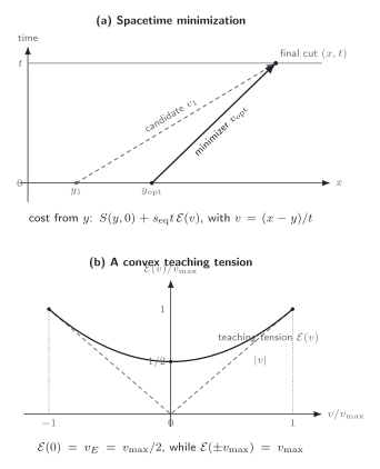
The one-dimensional membrane law is a minimization over the starting cut $y$: each straight segment has slope $v=(x-y)/t$ and total cost $S(y,0)+s_{\rm eq}t\mathcal E(v)$. The lower schematic shows the teaching tension $\mathcal E(v)=(v_{\max}^2+v^2)/(2v_{\max})$ on $|v|\leq v_{\max}$; it is convex, satisfies $\mathcal E(v)\geq|v|$, touches the effective cone at $\pm v_{\max}$, and has $v_E=\mathcal E(0)=v_{\max}/2$. The geometry and curve are schematic and not to scale; identifying $v_{\max}$ with $v_B$ needs an independent front check.

The cone constraints imply $v_E\leq v_{\max}$. Only after the endpoint is identified with an independently defined butterfly front does this become $v_E\leq v_B$. Neither form establishes an inequality involving every quasiparticle group velocity or the relativistic speed without further hypotheses. Mezei and Stanford 2017, §§ 2–4 explain why entanglement growth and the emergent information cone impose different constraints.

Local growth equation

The same variational law has a Hamilton–Jacobi form. Define the dimensionless entropy slope

$$\sigma(x,t)=\frac{1}{s_{\rm eq}}\frac{\partial S}{\partial x}.$$

Let $y_{\rm opt}$ be a unique interior minimizer and set $v_{\rm opt}=(x-y_{\rm opt})/t$. The envelope theorem differentiates the minimized value without differentiating $y_{\rm opt}$:

$$\partial_x S=s_{\rm eq}\mathcal E'(v_{\rm opt}), \qquad \partial_t S=s_{\rm eq}\!\left[ \mathcal E(v_{\rm opt})-v_{\rm opt}\mathcal E'(v_{\rm opt}) \right].$$

Thus $\sigma=\mathcal E'(v_{\rm opt})$, and where the coarse-grained solution is differentiable,

$$\frac{\partial S}{\partial t} =s_{\rm eq}\Gamma(\sigma), \qquad \Gamma(\sigma)=\min_v\bigl[\mathcal E(v)-v\sigma\bigr].$$

$\Gamma$ and $\mathcal E$ are Legendre-related descriptions of the same leading dynamics; the minus sign follows from $v=(x-y)/t$. In the locally equilibrated lattice normalization, subadditivity bounds the coarse-grained slope by $|\partial_xS|\leq s_{\rm eq}$, hence $|\sigma|\leq1$. A flat entropy profile has $\sigma=0$ and grows at $s_{\rm eq}\Gamma(0)=s_{\rm eq}v_E$. A steep initial profile can reduce the local production rate because the optimal membrane tilts and inherits more entropy from a neighboring cut.

For the parabolic teaching tension, minimization gives $v=v_{\max}\sigma$ for $|\sigma|\leq1$ and

$$\Gamma(\sigma)=\frac{v_{\max}}{2}(1-\sigma^2).$$

The vanishing at $|\sigma|=1$ expresses a slope bound in this normalization. It is not a diffusion equation: no second spatial derivative appears at leading deterministic order. Noise, higher gradients, or coupling to conserved fields can add subleading structure.

Fit one geometry and predict another

A reproducible finite-chain test isolates the zero-slope datum before attempting a full functional fit. Take the open tilted-field Ising chain used as a quantum-chaotic benchmark by Jonay, Huse, and Nahum 2018, Eq. (1), Figs. 5, 7, and 15–16,

$$H=\sum_{j=1}^{L-1}Z_jZ_{j+1} +0.5\sum_{j=1}^{L}Z_j -1.05\sum_{j=1}^{L}X_j,$$

with open boundaries, $L=16$, and $a=J=\hbar=1$. Start from $|{+y}\rangle^{\otimes L}$. Each displayed Hamiltonian term has zero expectation in this product state, so its energy density is exactly $e=0$. Because $H$ is traceless, this is the infinite-temperature energy density and independently fixes $s_{\rm eq}=\ln2$.

The training observables are the von Neumann entropies across the five central one-boundary cuts $x=6,\ldots,10$, evolved with a second-order Strang step $\Delta t=0.02$. On the frozen window $1.2\leq t\leq3.0$ in increments of $0.2$, their spread is below $2.3\times10^{-4}$ nats. That agreement is a boundary check, not five independent statistical samples. Least squares on their mean gives

$$S_{\rm cut}^{\rm fit}(t)=c+rt, \qquad c=-0.280139\ {\rm nats}, \qquad r=0.731256\ {\rm nats}/J^{-1},$$

with an RMSE of $0.02186$ nats. Therefore

$$v_E=\mathcal E(0)=\frac{r}{s_{\rm eq}}=1.05498.$$

Moving the lower and upper fit boundaries over $t_{\min}=1.0,1.2,1.4$ and $t_{\max}=2.8,3.0,3.2$ gives the systematic envelope $1.0405\leq v_E\leq1.0762$. These are deterministic, temporally correlated samples, so this range measures fit-window sensitivity rather than statistical confidence. The intercept corresponds to a microscopic delay $-c/r=0.3831$; it is a finite-time correction, not part of the asymptotic tension.

Now freeze $c$ and $r$. For a centered interval of length $\ell$, the two boundaries predict

$$S_\ell^{\rm pred}(t)= \operatorname{clip}\!\left(2(c+rt),\,0,\,\ell\ln2\right).$$

No interval entropy entered the fit. Here $S_{\rm dir}$ denotes the entropy obtained from the dense-state Strang evolution and a full-state coefficient-matrix SVD at the stated time step; it is a direct microscopic comparator, not exact continuous-time evolution. Schmidt probabilities below $10^{-14}$ are discarded before renormalization. For the held-out eight-site interval at the same exactly matched energy density, the ten times from $1.2$ through $3.0$ have RMSE $0.04351$ nats, maximum absolute error $0.07060$ nats, and signed mean residual $S_{\rm dir}-S_{\rm pred}=0.00216$ nats. At $t=3$, for example, $S_8^{\rm dir}=3.86172$ nats and the frozen prediction is $3.82726$ nats.

The figure separates this successful geometry transfer from two deliberate failures. Inspect the training residuals in panel (a), then compare the chaotic and integrable eight-site curves against the same frozen band in panel (b).

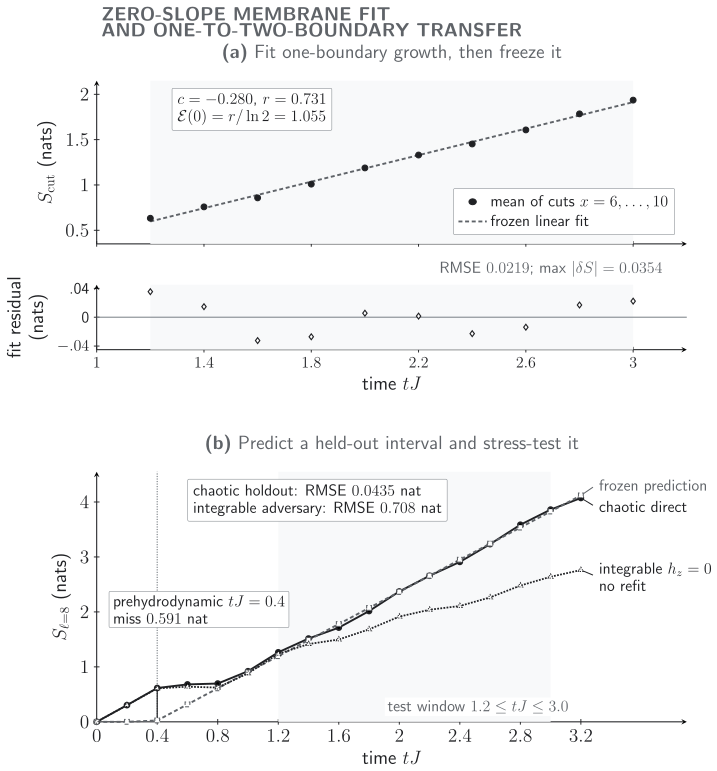
Fit, freeze, predict, and falsify at fixed energy density. (a) For the open $L=16$ tilted-field Ising chain, the five central single-cut entropies of $|{+y}\rangle^{\otimes16}$ determine $c=-0.280139$ nats and $r=0.731256$ nats per unit time on $1.2\leq t\leq3.0$; the dashed residuals remain within $0.03538$ nats. (b) Doubling the frozen one-boundary law predicts the held-out $\ell=8$ interval with RMSE $0.04351$ nats, whereas the same law applied without refitting to the integrable $h_z=0$ chain has RMSE $0.7080$ nats and misses the $t=3$ value by $1.1877$ nats. The separate $t=0.4$ chaotic point also misses the clipped extrapolation by $0.5910$ nats. The plot is quantitative at the stated lattice sizes and time steps; it tests $\mathcal E(0)$ and one-to-two-boundary transfer, not the curvature or endpoint of the full tension.

Download the quantitative SVG, CSV training, prediction, and control data, and JSON parameters, fit envelope, diagnostics, and claim boundary.

The timestep and algebraic controls are far smaller than the scientific residuals. Halving $\Delta t$ changes the central-cut entropy by at most $1.32\times10^{-4}$ nats and the eight-site entropy by at most $2.03\times10^{-4}$ nats. Across all four runs the norm error stays below $2.5\times10^{-13}$ and the complement-entropy mismatch below $8.9\times10^{-16}$ nats. For the chaotic $L=16$ run, the maximum energy-density drift falls from $3.69\times10^{-4}$ at $\Delta t=0.02$ to $9.23\times10^{-5}$ at $\Delta t=0.01$. Raising $L$ from $16$ to $18$ changes the central-cut entropy by at most $3.19\times10^{-5}$ nats and the held-out eight-site entropy by at most $0.04016$ nats. That interval-size shift is comparable to the $0.04351$-nat held-out RMSE, so the successful transfer is a controlled finite-chain result, not evidence that finite-size effects have disappeared.

This is intentionally a zero-slope test. A homogeneous product state determines $s_{\rm eq}\mathcal E(0)$, not the curvature of $\mathcal E(v)$ or $v_{\max}$. A full tension extraction needs nonzero-slope operator-entanglement cuts, an inhomogeneous initial entropy profile, or another independent geometry. Calling the affine fit a determination of the whole function would exceed the data.

Entanglement hydrodynamics is not charge hydrodynamics

The word “hydrodynamic” appears in two related but distinct senses.

Entanglement hydrodynamics is the long-wavelength evolution of $S(x,t)$ through $\Gamma$ or $\mathcal E$. Its field is an entropy profile over cuts, and it need not correspond to a conserved density.

Conserved-charge hydrodynamics begins from a continuity equation,

$$\partial_t n+\partial_x j=0,$$

with constitutive data such as $j=-D\partial_x n$. The charge profile can diffuse while the leading state entanglement grows ballistically. Conversely, an inhomogeneous conserved density can make the local equilibrium entropy density and effective tension position- and time-dependent, so the entropy profile need not obey the homogeneous law.

In a controlled local-equilibrium ansatz, first solve the conserved-density hydrodynamics, then evaluate a position- and time-dependent membrane on that background. This leading construction does not by itself imply that the membrane backreacts on the hydrodynamic fields. Do not label $v_E$ a diffusion speed or infer $D$ from a linear entropy slope. Mezei and Virrueta 2020, §§ 2–3 discuss this geometric coupling in holographic quench backgrounds.

Regime and failure controls

The same calculation supplies two no-refit adversaries.

Class transfer fails. Set the longitudinal field to zero, making the transverse-field Ising chain integrable, but keep $L=16$, $|{+y}\rangle^{\otimes16}$, $e=0$, $s_{\rm eq}=\ln2$, and the chaotic values of $c$ and $r$. For the eight-site interval the no-refit RMSE rises from $0.04351$ to $0.7080$ nats. At $t=3$, the integrable entropy is $2.63954$ nats rather than the predicted $3.82726$ nats, a signed residual of $-1.18772$ nats. The failed hypothesis is dynamical class: persistent mode occupations replace the locally mixing chaotic entropy current. Energy matching and numerical accuracy remain intact.

Early-time extrapolation fails. In the original chaotic chain at $t=0.4$, the direct full-state eight-site entropy is $0.61571$ nats. Clipping the frozen affine extrapolation at zero gives only $0.02473$ nats. The failed hypothesis is scale separation: the state is still in its microscopic entangling transient, before the fitted coarse-grained law applies.

Strongest surviving claim. On the measured $L=16$ window $1.2\leq t\leq3.0$, one fitted zero-slope entropy-production datum transfers from five central one-boundary cuts to a centered eight-site interval in this nonintegrable chain. It is not a full extraction of $\mathcal E(v)$, a microscopic evolution law, a continuum result, or a class-independent prediction.

Further applications should still move $t_{\min}$, vary $L$ and the region, and diagnose local equilibration independently of the entropy residual. Failure only for short intervals can reveal gradient or crossover corrections; failure across well-separated geometries rejects the proposed scaling window.

Separate mean growth and fluctuations. In noisy one-dimensional circuits, KPZ fluctuations scale as $t^{1/3}$ around a mean linear law. A deterministic Hamiltonian need not share that stochastic exponent. State which ensemble and statistic are being fitted.

Vary conserved-density profiles. A domain wall can couple slow charge relaxation to the entropy surface. If one homogeneous tension is retained, the local thermodynamic inputs and their evolution must still be supplied. The later fronts and velocities and integrable-versus-chaotic comparison pages provide independent diagnostics for the two hypotheses tested here.

The chapter orientation map shows that the membrane is an optional effective branch rather than a compulsory step. Its failure controls separate prehydrodynamic fitting from class transfer, and the diagnostic comparison records what a membrane fit actually reports.

Common pitfalls

Equating the membrane endpoint $v_{\max}$ with $v_B$. The Legendre structure fixes $v_{\max}$ inside the membrane model, while $v_B$ comes from an independently defined operator front. Equate them only after checking the front-identification hypothesis; neither speed is generally equal to $v_E$.

Calling a quasiparticle formula a membrane. Both can be variational-looking and produce linear growth, but their microscopic inputs and failure modes differ. Test integrability and out-of-sample geometry.

Using “hydrodynamic” without naming the field. State whether the evolving object is an entropy profile, a conserved density, or a coupled system.

Exercises

For the parabolic tension

$$\mathcal E(v)=\frac{v_{\max}^2+v^2}{2v_{\max}},$$

verify the standard endpoint conditions and prove $\mathcal E(v)\geq|v|$.

Solution

At $v=0$, $\mathcal E(0)=v_{\max}/2$, so $v_E=v_{\max}/2$. At $v=v_{\max}$,

$$\mathcal E(v_{\max})=v_{\max}, \qquad \mathcal E'(v_{\max})=\frac{v_{\max}}{v_{\max}}=1.$$

Finally,

$$\mathcal E(v)-|v| =\frac{(v_{\max}-|v|)^2}{2v_{\max}}\geq0.$$

Derive $\Gamma(\sigma)$ for the same tension when $|\sigma|\leq1$.

Solution

Minimize

$$f(v)=\frac{v_{\max}^2+v^2}{2v_{\max}}-v\sigma.$$

The stationary point satisfies $f'(v)=v/v_{\max}-\sigma=0$, so $v=v_{\max}\sigma$, which lies on the physical branch for $|\sigma|\leq1$. Substitution gives

$$\Gamma(\sigma)=\frac{v_{\max}}{2}(1-\sigma^2).$$

Use the fitted values $c=-0.2801386$ nats and $r=0.7312563$ nats per unit time to predict the centered eight-site entropy at $t=3$. Compare with the held-out direct-evolution value $S_8^{\rm dir}=3.8617225$ nats. Was this point used to determine either fit parameter?

Solution

The frozen two-boundary prediction is below both clipping limits, so

$$S_8^{\rm pred}(3)=2(c+3r)=3.8272608\ {\rm nats}.$$

The signed residual is therefore

$$S_8^{\rm dir}-S_8^{\rm pred}=0.0344616\ {\rm nats}.$$

No interval entropy was used in the fit: $c$ and $r$ came only from one-boundary cuts. This is why the comparison tests transfer to a held-out geometry rather than goodness of fit on the training observable.

At $t=0.4$, evaluate the same clipped prediction and compare it with the direct-evolution result $S_8^{\rm dir}=0.6157101$ nats. What assumption fails? Then explain why the matched-energy integrable calculation is a logically different adversary.

Solution

Here $2(c+rt)=0.0247279$ nats, already inside the clipping range. The residual is

$$0.6157101-0.0247279=0.5909822\ {\rm nats}.$$

The Hamiltonian is unchanged, but the time lies before the fitted scaling window, so the failed assumption is late-time scale separation. In the integrable adversary the time window is retained and the longitudinal field is changed to $h_z=0$; that test instead rejects transfer of one chaotic, locally equilibrating entropy-production law across dynamical classes.

A homogeneous half-chain entropy grows with slope $0.36$ per unit time. An independent thermodynamic calculation gives $s_{\rm eq}=0.8$. What membrane datum is determined? Can the full tension be inferred?

Solution

For a single cut, $dS/dt=s_{\rm eq}\mathcal E(0)$, so

$$v_E=\mathcal E(0)=\frac{0.36}{0.8}=0.45.$$

Only the value at zero slope is determined. The curvature, endpoint speed, and full $v$ dependence require inhomogeneous profiles, operator-entanglement data, or other geometries. Infinitely many convex tensions share $\mathcal E(0)=0.45$.

References

• Fisher, Matthew P. A., Vedika Khemani, Adam Nahum, and Sagar Vijay. “Random Quantum Circuits.” Annual Review of Condensed Matter Physics 14 (2023): 335–379. DOI.
• Jonay, Cheryne, David A. Huse, and Adam Nahum. “Coarse-Grained Dynamics of Operator and State Entanglement.” arXiv:1803.00089 (2018). arXiv.
• Mezei, Márk. “Membrane Theory of Entanglement Dynamics from Holography.” Physical Review D 98 (2018): 106025. DOI.
• Mezei, Márk, and Douglas Stanford. “On Entanglement Spreading in Chaotic Systems.” Journal of High Energy Physics 2017, no. 5 (2017): 065. DOI.
• Mezei, Márk, and Julio Virrueta. “Exploring the Membrane Theory of Entanglement Dynamics.” Journal of High Energy Physics 2020, no. 2 (2020): 013. DOI.
• Nahum, Adam, Jonathan Ruhman, Sagar Vijay, and Jeongwan Haah. “Quantum Entanglement Growth under Random Unitary Dynamics.” Physical Review X 7 (2017): 031016. DOI.
• Rampp, Michael A., Suhail A. Rather, and Pieter W. Claeys. “Entanglement Membrane in Exactly Solvable Lattice Models.” Physical Review Research 6 (2024): 033271. DOI.
• Zhou, Tianci, and Adam Nahum. “Entanglement Membrane in Chaotic Many-Body Systems.” Physical Review X 10 (2020): 031066. DOI.