Mutual Information and Regulator-Independent Correlations

Mutual information is the relative entropy between a joint state and the product of its marginals, so it measures every correlation visible to two declared algebras. For separated QFT regions it is finite and regulator independent only when two logically distinct requirements hold: the marginal product defines a normal state on the joint algebra, and the resulting relative entropy is finite. A matched regulator can instead establish the same conclusion by a controlled continuum limit at fixed positive separation. Under either route, mutual information bounds all bounded connected correlators, but it is not by itself a measure of quantum entanglement.

Required background. Use Relative Entropy for QFT States. Helpful background. Cluster decomposition supplies large-separation intuition, while regulated subregion entropy explains local ultraviolet terms.

Use the chapter’s task-comparison table to distinguish total correlation from entanglement, conditional correlation, recovery error, and channel distance.

Product states for separated algebras

Let $\mathfrak A$ and $\mathfrak B$ be commuting von Neumann algebras on a Hilbert space, let

$$\mathfrak M=\mathfrak A\vee\mathfrak B,$$

and let $\omega$ be a normal state on $\mathfrak M$. Its restrictions $\omega_A$ and $\omega_B$ always define an abstract normal product functional on the spatial tensor product $\mathfrak A\mathbin{\bar\otimes}\mathfrak B$. That fact alone does not put the product state on $\mathfrak M$.

The exact state-dependent hypothesis is the existence of a normal state $\varphi_\times$ on $\mathfrak M$ such that

$$\varphi_\times(ab)=\omega_A(a)\omega_B(b), \qquad a\in\mathfrak A,\quad b\in\mathfrak B.$$

If this normal product extension exists, it is unique because finite sums of products $ab$ are weakly dense in $\mathfrak M$. Algebraic mutual information is then the extended-valued Araki relative entropy

$$I_\omega(\mathfrak A{:}\mathfrak B) =S_{\mathfrak M}(\omega\Vert\varphi_\times) \in[0,+\infty].$$

The split property is a useful state-independent sufficient condition for this first requirement. The pair is split when a type-I factor $\mathfrak N$ satisfies

$$\mathfrak A\subset\mathfrak N\subset\mathfrak B'.$$

Then multiplication extends to a spatial normal isomorphism

$$\mathfrak A\mathbin{\bar\otimes}\mathfrak B \simeq \mathfrak A\vee\mathfrak B, \qquad a\otimes b\longmapsto ab,$$

and every pair of normal marginal states has a normal product extension. This is the operator-algebraic form of independent state preparation for separated laboratories Doplicher and Longo 1984, §§ 1–2; Fewster 2016, § 2, eqs. (2)–(8).

Split factorization does not imply that $I_\omega$ is finite. Even on $B(\ell^2)\mathbin{\bar\otimes}B(\ell^2)$, a faithful normal state can have infinite classical mutual information if its correlated probabilities have a sufficiently heavy tail. The split property constructs the reference state; finiteness is an additional analytic or phase-space condition.

One sufficient QFT theorem starts from a standard split pair of hyperfinite factors and a standard vector $\Omega$. With

$$\Xi_A(a)=\Delta_{B'}^{1/4}a\Omega, \qquad \Xi_B(b)=\Delta_{A'}^{1/4}b\Omega,$$

define $z_p=\min\{\lVert\Xi_A\rVert_p,\lVert\Xi_B\rVert_p\}$. If $z_p<\infty$ for some $0<p<1$, modular $p$-nuclearity gives

$$I_\omega(\mathfrak A{:}\mathfrak B) \leq \frac{z_p}{(1-p)e} +\eta(z_p-1)-\eta(z_p)<\infty, \qquad \eta(t)=-t\ln t.$$

The precise hypotheses and bound are Panebianco and Wegener 2022, Definition 13 and Theorem 25, eq. (21). Quasi-free Hadamard states of the real free scalar field satisfy the relevant modular $\ell^p$ condition for every $p>0$ Lechner and Sanders 2016, Definition 2.4 and §§ 3–5. These results do not remove the need to check standardness, hyperfiniteness, separation, and the chosen local algebras in an application. The rigorous noncommutative treatment develops the infinite-dimensional divergence machinery.

With a type-I regulator, $\varphi_\times=\rho_A\otimes\rho_B$ and the same definition becomes

$$I(A{:}B) =D(\rho_{AB}\Vert\rho_A\otimes\rho_B) =S(\rho_A)+S(\rho_B)-S(\rho_{AB}).$$

The last expression is safe only when all three density operators use the same regulator, algebra, boundary prescription, and center convention. Individual entropy divergences may then cancel in the complete combination, but that cancellation is evidence about the chosen limiting sequence, not a substitute for an algebraic finiteness theorem.

The structural map shows where the product comparison enters. Inspect the correlation branch: testing, recovery, and channel distances require different reference objects and resources.

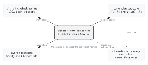
Mutual information is relative entropy to the normal product of the two marginal states. The diagram separates this total-correlation question from hypothesis testing, overlap, recovery, and channel comparison, each of which needs additional data. Schematic.

The exact connected-correlation bound

Use natural logarithms. Pinsker’s inequality for normal states on a von Neumann algebra is

$$S_{\mathfrak M}(\omega\Vert\varphi_\times) \geq \frac12\lVert\omega-\varphi_\times\rVert_*^2,$$

where $\lVert\cdot\rVert_*$ is the predual norm. In a type-I representation it is the trace norm of the density-operator difference; the trace distance is one half of this norm.

For bounded $X\in\mathfrak A$ and $Y\in\mathfrak B$, set $\delta=\omega-\varphi_\times$. Product factorization gives

$$\delta(XY)=\omega(XY)-\omega(X)\omega(Y).$$

Duality of the predual and operator norms, followed by submultiplicativity, gives

$$\begin{aligned} \bigl\lvert\omega(XY)-\omega(X)\omega(Y)\bigr\rvert &=\lvert\delta(XY)\rvert\\ &\leq\lVert\delta\rVert_*\lVert XY\rVert\\ &\leq\lVert\delta\rVert_*\lVert X\rVert\lVert Y\rVert. \end{aligned}$$

Combining the two inequalities yields the exact natural-log bound

$$\boxed{ I_\omega(\mathfrak A{:}\mathfrak B) \geq \frac{\bigl\lvert\omega(XY)-\omega(X)\omega(Y)\bigr\rvert^2} {2\lVert X\rVert^2\lVert Y\rVert^2}}$$

or, equivalently,

$$\bigl\lvert\langle XY\rangle_c\bigr\rvert \leq\sqrt{2I_\omega(\mathfrak A{:}\mathfrak B)} \,\lVert X\rVert\lVert Y\rVert.$$

For logarithms to base $b$, the lower-bound coefficient is $1/(2\ln b)$; in bits it is $1/(2\ln2)$. This is the von Neumann-algebra version of the many-body bound in Wolf et al. 2008, eq. (5), p. 070502-2.

The boundedness hypothesis is essential. A smeared field $\phi(f)$ is generally an unbounded operator, so inserting it directly into this operator-norm inequality is meaningless. Use a bounded function such as a Weyl unitary $e^{it\phi(f)}$ or $\sin[t\phi(f)]$, or prove a separate moment bound with explicit domain assumptions. Small mutual information forces every bounded connected correlator to be small; the converse does not follow from checking only a few correlators because they need not determine the joint state.

Finally, $I=0$ means that the joint state equals its product reference, but $I>0$ does not identify the correlation as quantum. For example, the separable state

$$\rho_{AB}=\sum_i p_i\lvert i,i\rangle\!\langle i,i\rvert$$

has $I(A{:}B)=-\sum_i p_i\ln p_i$ while containing only a shared classical label. Mutual information is total correlation, not an entanglement witness or a distillation rate.

Massive free scalar: two intervals and a bounded probe

Consider the ground state of the periodic harmonic chain

$$H=\frac12\sum_{n=0}^{N_{\rm box}-1} \left[ p_n^2+m^2q_n^2+\frac{(q_{n+1}-q_n)^2}{a^2} \right], \qquad [q_n,p_j]=i\delta_{nj}.$$

Its normal-mode frequencies and equal-time covariance functions are

$$\omega_k^2=m^2+\frac4{a^2}\sin^2\!\frac{\pi k}{N_{\rm box}},$$ $$X_r=\frac1{2N_{\rm box}}\sum_k \frac{\cos(2\pi kr/N_{\rm box})}{\omega_k}, \qquad P_r=\frac1{2N_{\rm box}}\sum_k \omega_k\cos\frac{2\pi kr}{N_{\rm box}}.$$

For a set of sites $V$, restrict these matrices to $X_V$ and $P_V$. With vanishing $qp$ covariance, compute the symplectic eigenvalues from the symmetric positive matrix

$$\nu_j= \sqrt{\lambda_j\!\left(X_V^{1/2}P_VX_V^{1/2}\right)}.$$

In exact arithmetic this matrix has the same spectrum as $X_VP_V$, but the symmetric form is substantially safer in floating-point calculations.

and

$$S(V)=\sum_j \left[ \left(\nu_j+\frac12\right)\ln\left(\nu_j+\frac12\right) -\left(\nu_j-\frac12\right)\ln\left(\nu_j-\frac12\right) \right].$$

The covariance construction and entropy formula follow Casini and Huerta 2009, § 2.2.1, eqs. (47), (63), and (65)–(66), and § 3.1.8, eqs. (197)–(199).

Set $R=1$, $mR=1$, $N_A=R/a=48$, and $N_{\rm box}=768$, so $a=1/48$ and $L_{\rm box}/R=16$. Region $A$ consists of 48 consecutive sites. After a gap of $N_L=L/a$ sites, region $B$ consists of the next 48 sites. The positive mass removes the scalar zero-mode ambiguity.

At $L/R=1$, the covariance calculation gives

$$S(A)=S(B)=1.27565791551736, \qquad S(A\cup B)=2.53799285328365,$$

and therefore

$$I(A{:}B)=2S(A)-S(A\cup B)=0.0133229777510748$$

nats at this regulator and volume.

To test the correlation inequality without using an unbounded field, define normalized block coordinates and local Weyl unitaries

$$Q_A=\frac1{\sqrt{N_A}}\sum_{j\in A}q_j, \qquad Q_B=\frac1{\sqrt{N_A}}\sum_{j\in B}q_j,$$ $$W_A(t)=e^{itQ_A}, \qquad W_B(-t)=e^{-itQ_B}.$$

Both unitaries have norm one. Write

$$V=\langle Q_A^2\rangle=\langle Q_B^2\rangle, \qquad C=\langle Q_AQ_B\rangle.$$

Because the ground state is centered and Gaussian and the two block coordinates commute,

$$\begin{aligned} \langle W_A(t)W_B(-t)\rangle&=e^{-t^2(V-C)},\\ \langle W_A(t)\rangle\langle W_B(-t)\rangle&=e^{-t^2V}. \end{aligned}$$

Thus the bounded connected correlator is

$$C_W(t)=e^{-t^2(V-C)}-e^{-t^2V} =t^2C+O(t^4),$$

which recovers the smeared field covariance in its small-$t$ coefficient. When $0<C<V$, this one-parameter lower bound is optimized by

$$t_*^2=\frac1C\ln\frac{V}{V-C}, \qquad I(A{:}B)\geq\frac12 C_W(t_*)^2.$$

At the stated $L/R=1$ benchmark,

$$V=0.268876636884024, \qquad C=0.0207784836978066,$$ $$t_*=1.96742110539313, \qquad C_W(t_*)=0.0295799193657355,$$

so Pinsker gives the strict same-regulator comparison

$$I(A{:}B)\geq 0.000437485814841707.$$

The bound is not expected to saturate because one pair of Weyl operators samples only part of the joint state. Its value is nevertheless nonzero, rigorous for the regulated Gaussian state, and more than an order of magnitude below the directly computed mutual information, as required.

Varying only the gap gives the separation test:

$L/R$	gap sites $N_L$	$I(A{:}B)$ (nats)	optimized Weyl lower bound
$0.25$	$12$	$0.131241716426838$	$0.00384770402808667$
$0.50$	$24$	$0.0544266662412567$	$0.00175428199307200$
$1.00$	$48$	$0.0133229777510748$	$0.000437485814841707$
$2.00$	$96$	$0.00116135423439179$	$0.0000368870395701559$
$4.00$	$192$	$0.0000129536349549042$	$0.000000397561546591766$

Both quantities decay as the intervals separate, while the lower bound remains below the full mutual information at every sampled gap. This finite set of points demonstrates the inequality and the expected clustering trend; it does not determine an asymptotic exponent.

For the fixed geometry $L/R=1$, a linear extrapolation in $(a/R)^2$ using $N_A\in\{16,24,32,48\}$ gives

$$I_{a\to0}=0.0133221488213132.$$

Refitting only the finest three resolutions changes the intercept by $7.50463567712745\times10^{-8}$. Repeating the extrapolation at $L_{\rm box}/R=12$ changes it by $1.21486215685918\times10^{-6}$. Their sum,

$$1.28990851363045\times10^{-6},$$

is an operational resolution-and-volume sensitivity envelope, not a statistical confidence interval or a rigorous bound on every omitted effect. At the finest point, the global covariance check has maximum residual $3.40\times10^{-14}$ from $XP=\mathbf 1/4$; the largest reported symplectic-eigensolver reconstruction residual is $8.79\times10^{-14}$, and eigenvalues below $1/2$ by at most $6.83\times10^{-12}$ are treated as roundoff. These arithmetic diagnostics are separate from the cutoff and volume variations. The raw values, covariance probes, gap sweep, and convergence fields are collected in the machine-readable benchmark record. A continuum local-algebra version should replace the sharp lattice top hat by a smooth compactly supported smearing, or prove the relevant approximation; one should not simply reuse the lattice operator without this domain check.

Contact, centers, and the strongest surviving claims

The validity map separates three ingredients that are easy to conflate: geometric separation, a fixed algebra and center, and one matched limiting procedure. Inspect the failure arrows before interpreting a finite number as an intrinsic continuum quantity.

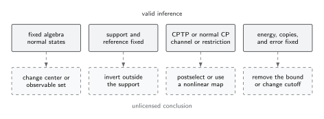
Positive separation and fixed algebras support the split or controlled-regulator routes. Bringing boundaries into contact can destroy split factorization and generate a new short-distance divergence; changing a center changes the observable algebra and product reference; mismatched entropy terms do not define one mutual information. Schematic.

Contact test. At every finite lattice spacing, adjacent blocks still have a type-I mutual information, and positivity and the bounded-operator Pinsker inequality remain exact. The continuum claim is weaker. When the physical gap $L$ is taken to zero, a new shared-boundary divergence appears; for sharp continuum algebras, the split inclusion may also fail. Therefore the strongest general statement at contact is finite-regulator positivity and correlation control. A finite regulator-independent continuum limit requires a new theorem or subtraction prescription and cannot be inherited from the $L>0$ calculation.

Changed-center test. In a gauge theory, adjoining or removing boundary-flux projectors changes the local von Neumann algebras. It can add or remove an ordinary classical mutual-information term carried by superselection labels. The associated product state, allowed bounded probes, and numerical value all change. Pinsker remains true separately for each fixed algebra with a normal product reference, but values obtained with different centers are not two regulators for the same quantity and should not be extrapolated together.

Mismatched-regulator test. If $S(A)$, $S(B)$, and $S(A\cup B)$ use different cutoffs or boundary prescriptions, their local counterterms need not cancel. Positivity of the resulting subtraction is not guaranteed because it is not the relative entropy of one regulated state against one product reference. The remedy is to recompute all three terms in one common scheme before taking any limit.

Compact CFT bridge

For ordered intervals of lengths $\ell_A$ and $\ell_B$ separated by $\delta>0$, define

$$x=\frac{\ell_A\ell_B} {(\ell_A+\delta)(\ell_B+\delta)}, \qquad 0<x<1.$$

For the vacuum of a full massless Dirac field in $1+1$ dimensions, the two chiral contributions give the exact result

$$I(A{:}B)=-\frac13\ln(1-x) =\frac13\ln \frac{(\ell_A+\delta)(\ell_B+\delta)} {\delta(\ell_A+\ell_B+\delta)}.$$

The chiral algebraic formula and its finiteness are proved in Longo and Xu 2018, Definition 3.17 and Theorem 3.18, p. 159. At large separation, $x\to0$ and $I=x/3+O(x^2)$. At contact,

$$I(A{:}B)=\frac13\ln \frac{\ell_A\ell_B}{\delta(\ell_A+\ell_B)} +O\!\left(\frac{\delta}{\ell_A}+\frac{\delta}{\ell_B}\right),$$

so the separated finite answer diverges as $\delta\to0^+$.

In a general CFT, the two-interval answer is not fixed by the central charge. A twist-field four-point function contains theory-dependent operator data Calabrese, Cardy, and Tonni 2009, § 1, eqs. (4)–(5), and § 5, eq. (81). At small $x$, the leading power is set by the smallest allowed sum of replica-theory scaling dimensions with vacuum quantum numbers; it is often $2\Delta_{\min}$, but selection rules and OPE coefficients matter Cardy 2013, abstract and § 2. The detailed geometry, replica expansion, and exact interval analysis belong to Mutual Information for Disjoint Regions.

Common pitfalls

Conflating existence with finiteness. A normal product extension makes $I_\omega$ an extended relative entropy; it can still equal $+\infty$. Split is sufficient for normal factorization, while modular nuclearity or a controlled regulator limit supplies the additional finiteness information.

Using an unbounded field in Pinsker. The displayed norm bound applies to bounded algebra elements. Replace a field by a Weyl unitary or another bounded functional calculus before invoking it.

Reading the Weyl bound as an estimate of the answer. It is a certified lower bound from one chosen probe family, not an approximation to the full mutual information.

Treating total correlation as entanglement. Shared classical labels contribute to mutual information. Distillable entanglement, negativity, and related measures require their own definitions and operational assumptions.

Exercises

1. Split factorization without finite mutual information. Let

$$p_n=\frac{c}{n(\ln n)^2},\qquad n\geq2,$$

where $c$ normalizes the distribution, and define

$$q_{ij}=(1-\varepsilon)p_i\delta_{ij}+\varepsilon p_ip_j, \qquad 0<\varepsilon<1.$$

Show that $q$ is a faithful normal state on a split type-I tensor product, has marginal distribution $p$ on both sides, and has infinite mutual information.

Solution

Every $q_{ij}$ is positive because the product term is positive, so the diagonal density operator has full support and defines a faithful normal state. Summing over either index gives

$$\sum_jq_{ij}=(1-\varepsilon)p_i+\varepsilon p_i\sum_jp_j=p_i.$$

For $i\neq j$, $q_{ij}/(p_ip_j)=\varepsilon$, whose total relative-entropy contribution is finite. On the diagonal,

$$q_{nn}\geq(1-\varepsilon)p_n, \qquad \frac{q_{nn}}{p_n^2}\geq\frac{1-\varepsilon}{p_n}.$$

The large-$n$ diagonal contribution is therefore bounded below, up to a finite constant, by

$$(1-\varepsilon)\sum_n p_n\ln\frac1{p_n}.$$

Since $p_n\ln(1/p_n)$ behaves as $1/[n\ln n]$, the sum diverges. Thus $D(q\Vert p\otimes p)=+\infty$ although the algebras are split and both states are faithful. Split supplied the normal product reference, not finiteness.

2. Optimize the Gaussian Weyl probe. For $0<C<V$, maximize

$$f(s)=e^{-s(V-C)}-e^{-sV},\qquad s=t^2\geq0,$$

and derive the value of $t_*$ used in the benchmark.

Solution

Differentiating gives

$$f'(s)=-(V-C)e^{-s(V-C)}+Ve^{-sV}.$$

The stationary-point equation is

$$e^{-sC}=\frac{V-C}{V},$$

and hence

$$s_*=\frac1C\ln\frac{V}{V-C}.$$

The function vanishes at $s=0$ and as $s\to\infty$, while it is positive in between, so this stationary point is the maximum. Substitution into Pinsker gives $I\geq f(s_*)^2/2$ because both Weyl operators have norm one.

3. Test the contact limit. Starting from the full-Dirac expression, find its leading behavior as $\delta\to0^+$ and explain which statement remains valid if one instead sets the lattice gap to zero before removing the cutoff.

Solution

Expanding the exact ratio at fixed positive $\ell_A,\ell_B$ gives

$$I(A{:}B)=\frac13\ln \frac{\ell_A\ell_B}{\delta(\ell_A+\ell_B)} +O\!\left(\frac{\delta}{\ell_A}+\frac{\delta}{\ell_B}\right).$$

It diverges logarithmically. If the gap is set to zero at finite lattice spacing, the regulated density matrices still define a nonnegative mutual information and the bounded-observable Pinsker bound still holds. What fails is the separated-region continuum finiteness claim: the new shared-boundary divergence and possible failure of split factorization require a different analysis.

4. Change a central observable. Suppose both local algebras contain a perfectly shared classical central label $z$ with probabilities $p_z$. Compute its contribution to mutual information. What happens if a new algebra convention removes that label from both observable algebras and all remaining degrees of freedom factorize?

Solution

The joint classical distribution is $P(z_A,z_B)=p_z\delta_{z_Az_B}$, whereas the product of marginals is $p_{z_A}p_{z_B}$. Therefore

$$I(Z_A{:}Z_B) =\sum_zp_z\ln\frac{p_z}{p_z^2} =-\sum_zp_z\ln p_z.$$

If the new algebras do not contain the label and the remaining state factorizes, their mutual information is zero. Neither value is an error: they answer questions about different observable algebras. Pinsker applies within either fixed choice, but the two values cannot be combined as cutoff samples of one quantity.

References

• Calabrese, Pasquale, John Cardy, and Erik Tonni. “Entanglement Entropy of Two Disjoint Intervals in Conformal Field Theory.” Journal of Statistical Mechanics: Theory and Experiment (2009): P11001. DOI. Open preprint.
• Cardy, John. “Some Results on the Mutual Information of Disjoint Regions in Higher Dimensions.” Journal of Physics A: Mathematical and Theoretical 46 (2013): 285402. DOI. Open preprint.
• Casini, Horacio, and Marina Huerta. “Entanglement Entropy in Free Quantum Field Theory.” Journal of Physics A: Mathematical and Theoretical 42 (2009): 504007. DOI. Open preprint.
• Doplicher, Sergio, and Roberto Longo. “Standard and Split Inclusions of von Neumann Algebras.” Inventiones Mathematicae 75 (1984): 493–536. DOI.
• Fewster, Christopher J. “The Split Property for Quantum Field Theories in Flat and Curved Spacetimes.” Abhandlungen aus dem Mathematischen Seminar der Universität Hamburg 86 (2016): 153–175. DOI. Open preprint.
• Lechner, Gandalf, and Ko Sanders. “Modular Nuclearity: A Generally Covariant Perspective.” Axioms 5, no. 1 (2016): 5. DOI. Open preprint.
• Longo, Roberto, and Feng Xu. “Relative Entropy in CFT.” Advances in Mathematics 337 (2018): 139–170. DOI. Open preprint.
• Panebianco, Lorenzo, and Benedikt Wegener. “Modular Nuclearity and Entanglement Measures.” arXiv:2110.05823v3 (2022). DOI. Open preprint.
• Wolf, Michael M., Frank Verstraete, Matthew B. Hastings, and J. Ignacio Cirac. “Area Laws in Quantum Systems: Mutual Information and Correlations.” Physical Review Letters 100 (2008): 070502. DOI. Open preprint.