Why Continuum QFT Does Not Factorize Naively

A lattice bipartition is an honest tensor product of site Hilbert spaces. A sharp spatial cut in relativistic continuum QFT is generally different: the represented local algebra is typically type III, so it cannot be identified with all bounded operators on a regional Hilbert-space factor. The claim concerns the local realization of observables, not whether the global Hilbert space admits some abstract tensor-product isomorphism. This page makes that distinction precise, constructs the regulated oscillator-chain comparison, and gives a two-scale test that keeps the ultraviolet cutoff separate from a physical split collar.

Required background. Review tensor products and local observable nets. Helpful background. Reflection-positive lattice regulators supply a controlled type-I comparison, and restricted states separates restriction from partial trace.

Local algebras, not abstract Hilbert spaces

Let $O$ be a causally complete region and $O'$ its causal complement—the region spacelike separated from $O$. The naive factorization claim is not merely that two abstract Hilbert spaces can be written down. It asks for a unitary $U:\mathcal H\to\mathcal H_O\otimes\mathcal H_{O'}$ that represents the local pair as

$$\begin{aligned} U\mathfrak A(O)U^\dagger &=\mathcal B(\mathcal H_O)\otimes 1,\\ U\mathfrak A(O')U^\dagger &=1\otimes\mathcal B(\mathcal H_{O'}). \end{aligned}$$

The first equality alone would make $\mathfrak A(O)$ a type-I factor. It would contain minimal projections—nonzero projections with no smaller nonzero subprojection—and have the ordinary operator trace needed to write every normal regional state as a density matrix. In the vacuum representation of the standard local free Bose-field models studied by Araki, the non-type-I cases are instead type III Araki 1964, pp. 956–965. Broader type-$\mathrm{III}_1$ conclusions require additional assumptions about the theory, region, representation, and short-distance structure; “local algebras are type III” is not an assumption-free theorem about every model called a QFT. The neighboring page on type-III algebras develops this classification in more detail.

Type III means, in particular, that there are no nonzero finite projections and no nonzero faithful normal semifinite trace on the factor. A restricted normal state

$$\omega_O=\omega|_{\mathfrak A(O)}$$

still exists. In a concrete representation, every normal state has a generally nonunique positive trace-class representative on the ambient $\mathcal B(\mathcal H)$; in a suitable representation it may also be a vector state. What fails is a canonical regional density matrix $\rho_O$ obtained from a local tensor factor, together with an intrinsic formula $-\operatorname{Tr}\rho_O\log\rho_O$.

Microcausality does not repair the problem. The relation $[\mathfrak A(O),\mathfrak A(O')]=0$ says that the two algebras commute; it does not say that their multiplication map extends to a spatial tensor product, that either algebra equals the other’s full commutant, or that independently chosen normal states admit a normal product extension.

Ultraviolet entanglement across a sharp boundary is the physical symptom of the same short-distance structure, but entropy divergence is not by itself a proof of type III. Type-I systems can also have states of infinite entropy. The decisive obstruction here is the algebra type; the regulated entropy tells us how a particular approximation approaches that obstruction.

The structural map places the sharp local algebra beside the three controlled substitutes used below.

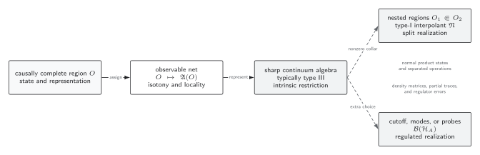
A causally complete region determines a sharp local algebra, usually type III. A nonzero split collar or an explicit cutoff, mode selection, or probe model can instead supply a type-I realization; these alternatives enable ordinary density matrices but retain different physical approximations. Schematic, not to scale.

What the legitimate substitutes supply

1. A lattice or finite-mode regulator. A finite collection of oscillators has a site or mode tensor product. Its reduced density matrix $\rho_A(a)$ and entropy $S_A(a)$ are exact at cutoff $a$, but the discretization, boundary rule, state, and limiting prescription remain part of the answer.
2. A split inclusion. For nested regions $O_1\Subset O_2$, when the inclusion is split there exists a type-I factor $\mathfrak N$ with $$\mathfrak A(O_1)\subset\mathfrak N\subset\mathfrak A(O_2).$$ The positive collar $O_2\setminus\overline O_1$ removes the coincident boundary. The construction permits normal product states and tensor-product methods, but $\mathfrak N$ is generally noncanonical and does not turn the sharp algebra into type I Doplicher and Longo 1984, pp. 493–496. Suitable nuclearity or phase-space conditions imply splitting in important classes of theories, but neither an arbitrarily thin collar nor every QFT is covered automatically Buchholz and Wichmann 1986, pp. 322, 325–328, 334–335.
3. Selected wavepackets or detectors. A finite collection of canonically independent modes defines a tensor-factor subsystem only after its commutator, or symplectic Gram matrix, has been checked and put in canonical form. Alternatively, detector ancillas and probe-generated operations define an operational subsystem without claiming that arbitrary overlapping field wavepackets are independent factors. Either choice can be nonlocal in position space and need not exhaust the observables of any geometric region.

These substitutes answer different questions. For a side-by-side statement of the conclusions each construction supports, use the chapter’s subsystem comparison table.

A reproducible oscillator-chain comparison

Discretize a real scalar field in $1+1$ dimensions as $N$ oscillators on a periodic ring of physical length $L=Na$, with $m>0$ to avoid the massless zero mode. Let $\phi_n$ and $\pi_n$ be lattice cell variables that approximate suitably averaged continuum fields near $x=na$, normalized by $[\phi_n,\pi_r]=i\delta_{nr}/a$. Define $q_n=\sqrt a\,\phi_n$ and $p_n=\sqrt a\,\pi_n$, so that $[q_n,p_r]=i\delta_{nr}$. With $q_{N+1}=q_1$, the regulated Hamiltonian is

$$H_a=\frac12\sum_{n=1}^{N} \left[p_n^2+m^2q_n^2+\frac{(q_{n+1}-q_n)^2}{a^2}\right] =\frac12p^{\mathsf T}p+\frac12q^{\mathsf T}K_aq,$$

with normal-mode frequencies

$$\Omega_r^2=m^2+\frac{4}{a^2}\sin^2\!\left(\frac{\pi r}{N}\right), \qquad r=0,\ldots,N-1.$$

For $N\ge3$, the circulant matrix has $(K_a)_{nn}=m^2+2/a^2$ and $(K_a)_{n,n\pm1}=-1/a^2$, with indices understood modulo $N$. The frequency formula is the safer definition for the exceptional $N=2$ ring, where the two neighboring bonds coincide.

The vacuum is Gaussian. Define $X_{nr}=\langle q_nq_r\rangle$ and $P_{nr}=\langle p_np_r\rangle$. Its position and momentum covariance matrices are

$$X=\frac12K_a^{-1/2}, \qquad P=\frac12K_a^{1/2}, \qquad \frac12\langle q_np_r+p_rq_n\rangle=0.$$

These covariance blocks follow directly by diagonalizing the positive quadratic form Audenaert et al. 2002, § II, pp. 2–3, after converting from their doubled-covariance convention $\gamma=2(X\oplus P)$.

For a contiguous block $A$ of $N_A$ sites, take the principal submatrices $X_A$ and $P_A$. The squared symplectic eigenvalues are the eigenvalues of the positive matrix $X_A^{1/2}P_AX_A^{1/2}$:

$$\nu_j^2\in\operatorname{spec}\!\left(X_A^{1/2}P_AX_A^{1/2}\right), \qquad \nu_j\ge\frac12.$$

The exact regulated entropy, in natural-log units, is then

$$\begin{aligned} S_A(a)&=\sum_{j=1}^{N_A}g(\nu_j),\\ g(\nu)&=\left(\nu+\frac12\right)\log\!\left(\nu+\frac12\right) -\left(\nu-\frac12\right)\log\!\left(\nu-\frac12\right). \end{aligned}$$

At the vacuum value $\nu=1/2$, interpret the second term by continuity, $0\log 0=0$.

This is a finite-$N$ covariance calculation in a type-I system, not an asserted continuum density matrix. Each oscillator Hilbert space is still infinite dimensional. The coupled-oscillator reduction and Gaussian entropy calculation go back to Bombelli et al. 1986, § II, pp. 374–378; the symplectic-spectrum form above is stated in Plenio et al. 2005, p. 3 after eq. (5), whose doubled-covariance eigenvalues are $\mu_j=2\nu_j$.

A reproducible refinement study fixes $mL$, the interval fraction $\ell/L=N_A/N$, the boundary condition, and the state, then repeats the calculation for $N,2N,4N,\ldots$. At each resolution:

1. diagonalize the real symmetric $K_a$ and record the smallest and largest $\Omega_r$;
2. verify the global purity identity $XP=\tfrac14 I_N$ using, for example, the matrix spectral residual $\lVert XP-\tfrac14 I_N\rVert_2$, and check $\min_j\nu_j\ge\tfrac12$ to the declared numerical tolerance;
3. compute $S_A(a)$ and smooth-field correlators such as those of $\Phi_a(f)=\sqrt a\sum_n f(na)q_n$ for test functions supported away from the boundary;
4. report resolution differences $Q(a/2)-Q(a)$ rather than hiding them inside a single decimal value.

There is no sampling uncertainty in this exact covariance calculation. The reported error budget instead consists of eigensolver precision, finite-volume effects, cutoff dependence, and any fit or extrapolation choice. If $m=0$, the periodic zero mode has no normalizable oscillator ground state, so a zero-mode or infrared prescription must be supplied before any entropy number is meaningful.

A separate critical benchmark

For the vacuum of a regulator tuned to a $1+1$-dimensional CFT on a circle, with one interval and $\ell,L-\ell\gg a$, a useful independent calibration is

$$S_A(a)=\frac{c}{3}\log\!\left[ \frac{L}{\pi a}\sin\!\left(\frac{\pi\ell}{L}\right) \right]+c_1'+o(1),$$

where $c$ is the central charge and $c_1'$ is regulator dependent Calabrese and Cardy 2004, § III, eq. (19). This CFT formula is not obtained by simply setting $m=0$ in the preceding noncompact periodic scalar chain: that limit still requires an explicit infrared and zero-mode prescription. The logarithm shows that a sequence of perfectly valid $\rho_A(a)$ need not approach a finite intrinsic sharp-region entropy. Its universal coefficient may survive even though the bare entropy does not.

Cutoff and collar are independent limits

Now choose nested intervals $O_1\Subset O_2$ with physical boundary separation $\delta>0$ at each boundary component. On a lattice, each boundary buffer contains approximately $k=\delta/a$ sites (about $2k$ in total for a two-sided interval). For finite-cutoff regions $R$ and $T$, write

$$I_a(R:T)=S_a(R)+S_a(T)-S_a(R\cup T)$$

for their mutual information in the regulated state. A valid two-parameter stress test uses a grid of cutoff spacings $a_i$ and physical collar widths $\delta_j$:

1. for each fixed $\delta_j$, refine $a_i\to0$, so the number of collar sites grows and $a_i/\delta_j\to0$;
2. check convergence of observables supported in $O_1$, observables supported in $O_2'$, and a separated diagnostic such as $I_{a_i}(O_1:O_2')$;
3. only after the fixed-$\delta$ continuum behavior is controlled, study what happens as $\delta_j\downarrow0$.

Holding the number of collar sites fixed while $a\to0$ instead gives $\delta=ka\to0$. It collapses the split distance at the same time as the ultraviolet cutoff and therefore cannot distinguish the two effects.

The adversarial comparison should also change the ultraviolet derivative stencil or entangling-cut prescription while keeping the physical infrared boundary condition, $mL$, $\ell/L$, $\delta/L$, and the continuum observables fixed. A separate boundary-condition scan tests infrared robustness; it is not a comparison of two regulators for the same finite-volume target. If smooth local expectations agree but the spectrum of $\rho_A(a)$ or its entropy changes without a controlled universal limit, the data do not support a regulator-independent density matrix. The strongest immediate statement is convergence on the specified observable class. Promote it to convergence of a restricted state only after controlling a convergence-determining class and topology; otherwise retain a fixed-collar split result or a specified universal combination—not an unqualified $\rho_A$.

What can survive regulator removal

Finite-cutoff object	Controlled continuum conclusion
$\operatorname{Tr}[\rho_A(a)A_a]$	May converge to $\omega_O(A)$ when the observables, states, and topology of convergence are specified.
The matrix $\rho_A(a)$ itself	Has no canonical sharp-region target because its carrier Hilbert space, regional factorization, and trace structure depend on the regulator.
$S_A(a)$	Is generally cutoff dependent; a universal coefficient, subtraction, relative entropy, or mutual information may have a controlled limit.
$I_a(O_1:O_2')$ at fixed $\delta>0$	Can provide a separated-region diagnostic, but convergence and infrared assumptions must be checked in the stated model.
A site-level minimal projector	Does not become a nonzero minimal projection of a type-III sharp local algebra.

Before drawing a continuum conclusion, use the validity map to keep the algebra, state, operation class, resources, and limiting prescription fixed.

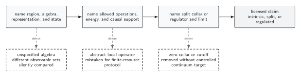
Every local-information claim must specify the represented algebra and state, the allowed operations and resource support, and any split collar or regulator. The dashed lower boxes show what fails when the algebra, protocol, or limiting prescription is left implicit. Schematic.

Common pitfalls

“The Hilbert space can be factorized, so the region factorizes.” An abstract isomorphism between separable Hilbert spaces does not say where the local algebras act. The required unitary must carry the represented local algebra to $\mathcal B(\mathcal H_O)\otimes1$, which its type-III structure forbids.

“Spacelike algebras commute, so they are independent tensor factors.” Commutation is necessary for compatible operations, but it does not imply a spatial tensor-product representation or normal product states. A split inclusion adds precisely the missing structure at positive separation.

“A divergent lattice entropy proves that the continuum algebra is type III.” It does not. The algebraic classification needs its own hypotheses and proof; the entropy divergence is a regulator-dependent diagnostic consistent with that classification.

“A density operator on the ambient Hilbert space is the regional density matrix.” Ambient implementations of a normal functional are generally nonunique. A regional reduced density matrix requires a specified type-I factorization or split realization.

“Four collar sites define the same split at every resolution.” Their physical width is $4a$, so the collar vanishes during refinement. Hold $\delta$ fixed first and let the number of collar sites grow.

Exercises

1. Two coupled oscillators. Consider

$$H=\frac12\left[p_1^2+p_2^2+\omega^2(q_1^2+q_2^2) +\kappa(q_1-q_2)^2\right], \qquad \omega>0,\quad\kappa\ge0.$$

Find the one-oscillator symplectic eigenvalue in the ground state and show that the two site factors are entangled exactly when $\kappa>0$.

Solution

With $q_\pm=(q_1\pm q_2)/\sqrt2$ and similarly for $p_\pm$, the normal-mode frequencies are $\Omega_+=\omega$ and $\Omega_-=\sqrt{\omega^2+2\kappa}$. Therefore

$$\langle q_1^2\rangle=\frac14\left(\frac1\omega+\frac1{\Omega_-}\right), \qquad \langle p_1^2\rangle=\frac14\left(\omega+\Omega_-\right),$$

and the mixed covariance vanishes. The reduced one-mode symplectic eigenvalue is

$$\nu=\sqrt{\langle q_1^2\rangle\langle p_1^2\rangle} =\frac14\sqrt{2+\frac{\Omega_-}{\omega}+\frac{\omega}{\Omega_-}}.$$

For $\kappa=0$, $\Omega_-=\omega$ and $\nu=1/2$, so $g(\nu)=0$. For $\kappa>0$, the arithmetic–geometric mean inequality gives $\Omega_-/\omega+\omega/\Omega_->2$, hence $\nu>1/2$ and $g(\nu)>0$. The factorization exists at this regulator; the ground state simply is not a product across it.

2. Diagnose a collapsed collar. A refinement study uses $a_n=L/2^n$ and removes exactly four sites between $O_1$ and $O_2'$. Does it test the split limit at fixed separation? Give a valid replacement protocol.

Solution

No. Its physical collar is $\delta_n=4a_n\to0$, so cutoff removal and collar collapse occur together. Choose physical widths $\delta_j>0$ first. For each $\delta_j$, take $k_{n,j}$ to be the nearest integer to $\delta_j/a_n$ and refine until $a_n/\delta_j$ and the observable residuals are small. Only then compare the fixed-$\delta_j$ limits as $\delta_j\downarrow0$.

3. State the strongest justified conclusion. Suppose two lattice discretizations give the same continuum limits for all tested smooth local correlators and for fixed-separation mutual information, while their $S_A(a)$ values differ by a cutoff-dependent boundary term. What may be claimed?

Solution

The data support agreement of the limiting expectation values on the tested observable class and a common fixed-separation information quantity within the tested errors. Unless that class is shown to determine states in a stated topology, they do not establish equality—or even existence—of complete continuum restricted-state limits. They also do not support a regulator-independent sharp-region density matrix or bare entropy. A universal entropy coefficient or subtraction may be claimed only after showing that the proposed combination agrees under both discretizations and has a controlled extrapolation.

References

• Araki, Huzihiro. “Type of von Neumann Algebra Associated with Free Field.” Progress of Theoretical Physics 32 (1964): 956–965. DOI.
• Audenaert, Koenraad, Jens Eisert, Martin B. Plenio, and Reinhard F. Werner. “Entanglement Properties of the Harmonic Chain.” Physical Review A 66 (2002): 042327. DOI.
• Bombelli, Luca, Rabinder K. Koul, Joohan Lee, and Rafael D. Sorkin. “Quantum Source of Entropy for Black Holes.” Physical Review D 34 (1986): 373–383. DOI.
• Buchholz, Detlev, and Eyvind H. Wichmann. “Causal Independence and the Energy-Level Density of States in Local Quantum Field Theory.” Communications in Mathematical Physics 106 (1986): 321–344. DOI.
• Calabrese, Pasquale, and John Cardy. “Entanglement Entropy and Quantum Field Theory.” Journal of Statistical Mechanics: Theory and Experiment 2004 (2004): P06002. DOI.
• Doplicher, Sergio, and Roberto Longo. “Standard and Split Inclusions of von Neumann Algebras.” Inventiones Mathematicae 75 (1984): 493–536. DOI.
• Plenio, Martin B., Jens Eisert, Jens Dreissig, and Marcus Cramer. “Entropy, Entanglement, and Area: Analytical Results for Harmonic Lattice Systems.” Physical Review Letters 94 (2005): 060503. DOI.