Entanglement, Correlation, and Hydrodynamic Fronts

A front is an inference from data, not a bright line that exists independently of measurement. A defensible front claim names the observable, matched control, threshold, error floor, crossing rule, fitting window, and held-out test. Entropy, mutual information, connected correlators, conserved density, and operator influence can then reveal different translation speeds and broadening laws without being compressed into one “information velocity.” Unless stated otherwise, entropy on this page means von Neumann entropy $S_1$ in nats.

Required background. Operator spreading and scrambling defines operator fronts, microcausality supplies the relativistic support condition, entanglement growth supplies entropy data, and mutual information supplies a finite correlation measure.

Helpful background. Membrane entanglement supplies the distinction between the entropy-production coefficient $v_E$ and the membrane endpoint $v_{\max}$.

From a named observable to an arrival

Let $G(x,t)$ be a measured diagnostic and $G_{\rm ctrl}(x,t)$ the result of a matched control evolved and sampled by the same procedure. The coordinate $x$ must be defined by the diagnostic: it can label an entropy cut, a detector position, or the separation between two finite regions. Retain the signed contrast

$$\Delta G(x,t)=G(x,t)-G_{\rm ctrl}(x,t)$$

for interpretation. If its sign oscillates, define a nonnegative arrival signal such as

$$Q(x,t)=|\Delta G(x,t)|$$

without discarding the signed data. A static control $G_{\rm ctrl}(x,0)$ is sufficient only when the control is stationary; otherwise it folds control dynamics into the alleged front.

For an absolute threshold $\eta$ above the propagated error floor, the first-arrival time is

$$t_\eta(x)=\inf\{t\geq t_{\rm first}:Q(x,t)\geq\eta\}.$$

Here $t_{\rm first}$ is the first trustworthy sample, not automatically the start of the asymptotic fitting window. A signal already above threshold at $t_{\rm first}$ is left-censored. A signal that never crosses by the final sample is right-censored. Neither case should be assigned an invented arrival time.

At fixed time, define $x_\eta(t)$ as the outermost crossing in the declared propagation direction. A profile can cross the same level more than once, so “outermost right-moving crossing” is part of the estimator. Interpolate only between the two samples bracketing that crossing, and propagate their uncertainty. The functions $t_\eta(x)$ and $x_\eta(t)$ are geometric inverses only for one monotone branch; fitting one and algebraically inverting the result generally changes the statistical problem.

An absolute threshold can move or disappear merely because an amplitude decays. A same-time relative threshold,

$$\frac{Q(x,t)}{\max_{x'\in\mathcal D}Q(x',t)}=\theta, \qquad 0<\theta<1,$$

removes an overall amplitude but introduces dependence on the spatial domain $\mathcal D$ and on a possibly noisy or split peak. Report several fixed $\theta$ values, the absolute error floor, interpolation rule, and persistence requirement. Threshold variation is a test of the claim, not an optional cosmetic choice.

Translation, broadening, and amplitude

A useful full-profile ansatz separates three effects:

$$G(x,t)=G_{\rm ctrl}(x,t)+A(t) F\!\left(\frac{x-x_0-v_ft}{w(t)}\right)+\cdots, \qquad w(t)=\Gamma t^\alpha.$$

$v_f$ translates the profile, $w(t)$ gives its width, $A(t)$ its amplitude, and $\Gamma$ carries units $L/T^\alpha$. Calling the front broadened ballistic requires

$$\frac{w(t)}{t}\longrightarrow0.$$

For the power law above this means $0<\alpha<1$. At a fixed profile level $F(z_\theta)$,

$$x_\theta(t)=x_0+v_ft+z_\theta\Gamma t^\alpha.$$

The $t^\alpha$ term is subleading only when $\alpha<1$. If $\alpha=1$, different thresholds can have different leading slopes; if $\alpha>1$, the ansatz does not describe a ballistic front. Define an asymptotic threshold-independent velocity only when

$$v_f=\lim_{t\to\infty}\frac{x_\theta(t)}{t}$$

exists and is stable over a nonzero threshold interval. Otherwise report the finite-time family $v_\theta(t)$ or the translation parameter of the fitted profile, not a unique front velocity.

Fit competing models on a predeclared training window, freeze every parameter and preprocessing choice, and compare predictions on later times. A smaller in-sample residual from a more flexible curve is not evidence for its scaling law. Move the training endpoints, vary the threshold, repeat at another size or regulator, and stop at the strongest statement that survives those changes.

Advection–diffusion separates drift from width

The normalized one-dimensional advection–diffusion kernel cleanly separates translation and broadening:

$$n(x,t)=\frac{1}{\sqrt{4\pi Dt}} \exp\!\left[-\frac{(x-ut)^2}{4Dt}\right].$$

At relative threshold $n(x_\theta,t)/n(ut,t)=\theta$, its two branches are

$$x_\theta(t)=ut\pm2\sqrt{Dt\ln(1/\theta)}.$$

The center translates at $u$, while the width grows as $\sqrt{Dt}$. Pure diffusion has $u=0$, so $x_\theta(t)/t\propto t^{-1/2}$ and no nonzero asymptotic front speed. With $D=0.7a^2/\tau$, $\theta=0.1$, and $u=0$,

$$x_{0.1}(2\tau)=2a\sqrt{1.4\ln10}\approx3.59088a, \qquad x_{0.1}(8\tau)\approx7.18177a.$$

The contour doubles when time is quadrupled. A constant-speed fit over a short interval is therefore window dependent. Infer $D$ from $x_\theta^2$ versus $t$, the profile variance, a constitutive response, or a small-momentum decay rate—not by renaming $\sqrt{D/t}$ as a velocity. The conservation-law treatment develops the hydrodynamic assumptions behind that inference.

The diffusion equation itself has an instantaneous Gaussian tail at every $x$ for every $t>0$. Its threshold contour is therefore not a boundary of exact support. Microscopic causal or lattice models can produce diffusion as a long-distance effective description while retaining a distinct causal or Lieb–Robinson constraint outside that regime.

Which speed did you measure?

Relativistic causal speed $c$. Point fields are operator-valued distributions, so the clean support statement uses smeared fields or bounded elements of local algebras:

$$[\mathcal O(f),\mathcal O'(g)]=0$$

when the supports of $f$ and $g$ are spacelike separated. This constrains intervention and commutator diagnostics. Vacuum and excited-state correlators need not vanish outside one another’s light cones.

Lieb–Robinson velocity $v_{\rm LR}$. For a finite-dimensional, short-range lattice Hamiltonian, a schematic bound is

$$\|[O_X(t),O_Y]\| \leq C N_{XY}\|O_X\|\|O_Y\| \exp\!\left[-\frac{d(X,Y)-v_{\rm LR}|t|}{\xi}\right].$$

$N_{XY}$ denotes a geometric factor such as the number of relevant interaction links between the supports. All constants depend on the interaction, graph, metric, support sizes, and proof. Different estimates can therefore give different valid $v_{\rm LR}$ values for the same model, usually above its observed fronts Lieb and Robinson 1972, Theorem 1; Bravyi, Hastings, and Verstraete 2006, Eqs. (1)–(2). Generic continuous-time short-range lattices have exponentially small tails rather than exact zeros, although finite-depth circuits can possess an exact discrete causal cone.

Group velocity $v_g(k)$. For $\varepsilon(k)=\hbar\omega(k)$,

$$v_g(k)=\frac{1}{\hbar}\frac{\partial\varepsilon(k)}{\partial k} =\frac{\partial\omega(k)}{\partial k}.$$

It moves a sufficiently narrow wave packet. A quench excites a distribution of momenta, so maximum, entropy-weighted, peak, and threshold velocities can differ.

Correlation-front speed $v_C$. This is a translation, peak, or threshold speed of a named correlator with a fixed state and operator choice. An operator orthogonal to the carried mode can show no visible front while another correlator responds.

Entanglement velocity $v_E$. In a locally equilibrated homogeneous regime, $dS_1/dt=s_{\rm eq}v_E|\partial A|$ defines a coarse-grained entropy-production coefficient. In the one-dimensional membrane convention of the preceding page,

$$v_E=\mathcal E(0), \qquad v_E\leq v_{\max}.$$

Here $v_{\max}$ is the membrane endpoint, not automatically a butterfly velocity. Only an independent operator-front identification permits $v_{\max}=v_B$ and hence the conditional comparison $v_E\leq v_B$ Zhou and Nahum 2020, §§ II–III.

Butterfly and task velocities. A commutator or regulated OTOC can define $v_B$; a decoder or recovery task can define still other arrivals. Those quantities are imported here only as comparators. Their definitions and non-equivalence belong to Information Velocities and Causal Bounds.

Correlation is not signaling

A state can contain correlations at arbitrary separation before the quench. Critical ground states, squeezed states, and the vacuum are familiar examples. Their mutual information or two-point function at $t=0$ is not a signal sent by the later protocol.

To test causal influence, compare deterministic trace-preserving local encoding channels $\mathcal E_a$ and $\mathcal E_{a'}$ applied to the same prior state and ask whether a receiver statistic changes:

$$\Delta_{a,a'}\langle O_B(t)\rangle =\langle O_B(t)\rangle_a-\langle O_B(t)\rangle_{a'}.$$

Microcausality constrains this intervention contrast. A conditional ensemble obtained by postselecting a local outcome can change at spacelike separation through steering, but without access to the outcome it cannot transmit a message. By contrast, $\langle O_AO_B\rangle_c$ and $I(A:B)$ quantify correlation in one state. A raw correlator subtraction is not itself a signaling measure. However, if “kick” and “no kick” are selectable deterministic local unitaries and the compared quantity is a receiver-local statistic, those alternatives do instantiate the encoding contrast above.

On a lattice, compare a measured contour with both the dispersion and a theorem that actually bounds the chosen diagnostic and initial-state class. An entropy or raw-correlation contour outside a quoted commutator estimate is not automatically a violation. The mismatch may instead show that the observable, unbounded local Hilbert space, interaction range, graph metric, or state assumptions lie outside the theorem.

Conservation splits the speed dictionary

A conserved density can spread diffusively while von Neumann entanglement remains ballistic. Kim and Huse 2013, abstract gives an explicit nonintegrable example with diffusive energy transport and linearly growing entanglement. Higher Rényi entropies can respond differently: in the one-dimensional diffusive systems studied by Rakovszky, Pollmann, and von Keyserlingk 2019, Eqs. (2)–(7), conserved-density fluctuations produce leading $\sqrt t$ growth for Rényi index greater than one while $S_1$ remains linear at leading order.

A conserved operator projection may diffuse while nonconserved weight develops a ballistic leading edge and a power-law hydrodynamic wake Khemani, Vishwanath, and Huse 2018, abstract and §§ II–IV; Rakovszky, Pollmann, and von Keyserlingk 2018, §§ II–IV. Conservation therefore does not impose one common “diffusion velocity.” Record the entropy order, operator overlap, density, current, and front definition before comparing exponents.

Exact local-kick front extraction

The worked application uses an open, half-filled free-fermion chain,

$$H=-J\sum_{j=0}^{L-2} \left(c_{j+1}^\dagger c_j+c_j^\dagger c_{j+1}\right), \qquad a=J=\hbar=1.$$

At $t=0$, a central site $j_0$ receives the deterministic local phase kick

$$U_\phi=e^{i\phi n_{j_0}}, \qquad \phi=\frac{\pi}{2},$$

and then evolves under the unchanged Hamiltonian. The matched control is the same half-filled ground state evolved without the kick, hence stationary. The infinite-chain dispersion supplies an independent band-velocity comparator,

$$\varepsilon(k)=-2J\cos(ka), \qquad v_{g,\max}=\max_k\frac{|\partial_k\varepsilon|}{\hbar} =\frac{2Ja}{\hbar}=2.$$

This $v_{g,\max}$ is the maximum quasiparticle group velocity and the asymptotic soft-edge comparator. It is not a hard support speed: continuous-time lattice evolution has small tails, and a finite-time low-threshold contour can lie beyond the ray $x=2t$ without contradicting the dispersion.

Let $G_{ij}=\langle c_i^\dagger c_j\rangle$. The full-chain ground-state $G_0$ is a projector, the kick changes it by rank at most two, and one-particle spectral evolution gives $G(t)$ without time stepping. Its restricted block $G_{A_x}$ is generally not a projector; its fractional eigenvalues are precisely what carry the entanglement across the cut. For $A_x=\{0,\ldots,j_0+x-1\}$,

$$S_1(A_x,t)=-\sum_m\left[ \nu_m\ln\nu_m+(1-\nu_m)\ln(1-\nu_m) \right].$$

The primary profiles are the cut-entropy contrast

$$\Delta S_x(t)=S_1(A_x,t)-S_1^{\rm ctrl}(A_x,t)$$

and the bounded nearest-neighbor connected-density contrast

$$\Delta C_x^{(nn)}(t)= \Delta\!\left[ \langle n_jn_{j+1}\rangle-\langle n_j\rangle\langle n_{j+1}\rangle \right] =-\Delta|G_{j,j+1}|^2.$$

The local density $\Delta n_j$ and rightward bond current $\Delta j_{j+1/2}=+2J\operatorname{Im}\Delta G_{j,j+1}$ provide observable adversaries. Both signed profiles and the nonlinear connected contrast are retained. For each diagnostic $Q$, its arrival is the outermost right-moving crossing of $|\Delta Q|$ at $\theta=0.02,0.05,0.10,0.20$ times that diagnostic’s same-time sampled peak, with log-linear interpolation between adjacent lattice coordinates.

The stored integer $x$ is a distance label, not one common geometric point for all four diagnostics. Density is sampled at $j_0+x$, bond quantities on $(j_0+x,j_0+x+1)$, and $A_x$ ends at $j_0+x-1$. These half-site offsets enter the observable-specific intercept $c$; comparing fitted slopes does not require pretending that the intercepts coincide.

The primary calculation uses $L=512$, $j_0=256$ in zero-based indexing, and exact samples $Jt/\hbar=12,16,\ldots,96$. At each time it samples $x=1,\ldots,16$ together with the integer band $2Jt/\hbar-22\leq x\leq2Jt/\hbar+22$. No smoothing is applied. Signals below $2\times10^{-13}$ are classified as numerically blind, and ordinary unweighted least squares fits the retained contours. The sample at $Jt/\hbar=12$ is an excluded early diagnostic; fits see only $16,20,\ldots,56$, while $60,64,\ldots,96$ are untouched. The three frozen candidates are

$$\begin{aligned} x_{\rm bal}(t)&=c+vt,\\ x_{\rm broad}(t)&=c+vt+g t^{1/3},\\ x_{\rm diff}(t)&=c+d\sqrt t. \end{aligned}$$

The $t^{1/3}$ candidate is motivated by soft-edge broadening in other free lattice fronts Hunyadi, Rácz, and Sasvári 2004, Eqs. (11)–(16); Eisler and Rácz 2013, Eqs. (5)–(12). It is tested here, not imported as the answer for this entropy contour. The covariance reduction follows Peschel 2003, Eqs. (5)–(12), while Eisler 2021, §§ 2 and 5 supplies the local particle–hole excess-entanglement framework rather than this exact phase-kick result. The finite primary energy injection is $1.27324157J$, approaching $4J/\pi$ in the infinite chain.

Frozen front prediction and a width adversary

For the primary entropy contour at $\theta=0.05$, the broadened-ballistic fit gives

$$v=1.98828135,$$

close to the independent $v_{g,\max}=2$ band edge. Its root-mean-square error on the ten untouched times is $0.01433$ lattice sites. The rigid ballistic fit has held-out error $0.05759$ sites, while the genuinely diffusive $c+d\sqrt t$ model misses by $18.4753$ sites. Thus the new data strongly distinguish ballistic translation from pure diffusion; the smaller improvement from the $t^{1/3}$ term must be judged together with the width test below.

The result is not an accident of one threshold. Across $\theta=0.02,0.05,0.10,0.20$, broadened-fit entropy velocities range from $1.98595$ to $1.99459$. At $\theta=0.05$, advancing fit windows $[12,44]$, $[16,56]$, $[20,64]$, $[24,72]$, and $[28,80]$ give $1.98609\leq v\leq1.98917$. These ranges are deterministic estimator-sensitivity envelopes, not statistical confidence intervals.

The figure separates the two questions that a visually sharp front can otherwise blur. In panel (a), inspect whether each frozen curve reaches the open held-out markers. In panel (b), compare the difference between a low and a high entropy threshold rather than fitting another leading slope.

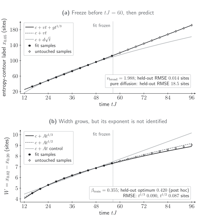
Exact finite-chain local-kick benchmark. For the open $L=512$ chain, $\phi=\pi/2$, and $\theta=0.05$, panel (a) shows the entropy-contour label $x_\theta$; filled circles were fitted over $16\leq Jt/\hbar\leq56$, and open diamonds were untouched over $60\leq Jt/\hbar\leq96$. The $c+vt+g t^{1/3}$ model has $v=1.98828$ and held-out RMSE $0.01433$ sites, compared with $0.05759$ for $c+vt$ and $18.4753$ for pure diffusion. Panel (b) shows $W=x_{0.02}-x_{0.20}$. Constant width and linear-in-$t$ widening have held-out RMSEs $2.28143$ and $0.69694$ sites, whereas $t^{1/3}$ and $t^{1/2}$ give $0.09015$ and $0.08670$ sites. The latter near-tie does not identify an exponent. This is a quantitative fixed-regulator result, not a support cone or continuum extrapolation; $v_{g,\max}=2$ is an asymptotic group-velocity comparator.

The width training scan selects $\beta=0.355$, while a scan chosen after seeing the held-out data would select $0.420$. The latter is a diagnostic, not a prediction. What survives is narrower: the entropy-contour width grows on this window, and both a rigid width and a linear fan fail, but $1/3$ versus $1/2$ is unresolved.

The $L=384$ size control runs only through $Jt/\hbar=64$, before the leading band approaches the boundary. Its $\theta=0.05$ entropy contour has RMSE $0.00875$ sites against $L=512$ and a maximum shift of $0.02258$ sites. Algebraic and numerical controls give direct-versus-rank-two covariance error below $8.9\times10^{-16}$, projector error below $1.3\times10^{-15}$, particle-number drift below $1.2\times10^{-15}$, and pure-state complement-entropy mismatch below $4.0\times10^{-14}$ nats.

Download the quantitative SVG, complete long-form CSV profiles, fits, and controls, compact CSV view used by the figure, and JSON calculation, schema, diagnostics, and claim boundary. The compact view is deterministically derived from the complete record; it does not add or refit a data point.

Observable, threshold, and window attacks

The scientific claim is not selected by the prettiest curve. The frozen adversary performs four changes.

• It repeats the contour at all four thresholds and across the five advancing windows listed above.
• It compares the entropy cut with connected nearest-neighbor density, local density, and bond current.
• It repeats the pre-boundary data through $Jt/\hbar=64$ at $L=384$.
• It changes the kick to $\phi=\pi$. At half filling this symmetry point blinds both local density and bond current even though entropy and connected-density signals remain active.

The last control is an exact warning against identifying “the front” with one convenient operator. With

$$|{\rm ph}\rangle=2\left(n_{j_0}-\frac12\right)|{\rm GS}\rangle,$$

the half-filled phase-kicked state is

$$U_\phi|{\rm GS}\rangle =e^{i\phi/2}\left[ \cos\!\frac\phi2\,|{\rm GS}\rangle +i\sin\!\frac\phi2\,|{\rm ph}\rangle \right].$$

At $\phi=\pi$, the ground-state component disappears. The bipartite particle–hole transformation $\mathcal Cc_j\mathcal C^{-1}=(-1)^jc_j^\dagger$ leaves $H$ invariant, maps $n_j$ to $1-n_j$, reverses the bond current, and sends $U_\pi$ to $-U_\pi$. The unique even-$L$ half-filled ground state, and therefore its $\pi$-kicked evolution, is invariant under $\mathcal C$ up to phase. Both one-point contrasts must consequently vanish: their largest recorded values are only $1.01\times10^{-15}$ and $1.08\times10^{-15}$, respectively, even though the entropy peak remains between $1.354$ and $1.379$ nats and the particle–hole-even connected-density response remains nonzero. A missing one-point response is therefore not a missing state perturbation.

The connected-density channel has a second, subtler limitation in the primary $\phi=\pi/2$ run. At the maximum-group-velocity edge, the leading phase-kick correction to $G_{j,j+1}$ is imaginary while the half-filled ground-state bond is real. Its contribution linear in the correction therefore cancels from $|G_{j,j+1}|^2$, leaving a weaker leading connected-density signal than the density or current. Same-time relative contours remain well defined, but equality of their amplitude exponents must not be assumed.

The observable comparison sharpens that conclusion. The bond-current contour at $\theta=0.10$ gives $v=1.99855320$ and held-out RMSE $0.03414$ sites. The connected-density contour at $\theta=0.20$ also has a near-edge ballistic slope, $v=2.00398136$, but is predictively noisy: its rigid-ballistic held-out RMSE is $0.66975$ sites, slightly better than the broadened model’s $0.70328$. The calculation therefore does not attribute resolved broadening to this connected channel.

The strongest conclusion supported by these checks is finite and diagnostic-specific: this exact regulated free-fermion quench has ballistically translating entropy and bond-current leading contours whose fitted slopes approach the independent maximum band group velocity, while the connected-density channel gives a noisier ballistic contour. On the tested time window, the entropy threshold width favors growing sublinear candidates over constant and linear controls. It does not determine a universal broadening exponent, a hydrodynamic or interacting velocity, $v_B$, a signaling speed, an exact support cone, or a continuum limit. In finite-bond-dimension MPO calculations of operator right-weight fronts, even a plausible exponential tail can coexist with errors in the peak and width, so convergence must cover the full fitted front Lopez-Piqueres et al. 2021, §§ II.2–II.3.

Scientific evidence cutoff: 26 August 2026. The research-sensitive front and broadening comparisons were checked through this date against the overview by Fisher et al. 2023, §§ 3–5. The alternating-initial-state free-fermion correlation front of Fujimoto and Sasamoto 2024, abstract supplies current context, not validation of this local phase kick.

Reproducibility and stop rule

A front analysis should preserve the following chain:

1. Archive signed profiles, the matched time-dependent control, coordinates, units, operator definitions, entropy order, and numerical or experimental error model.
2. Freeze smoothing, persistence, interpolation, threshold, censoring, boundary-exclusion, and fitting rules before examining held-out times.
3. Compare translation, broadening, diffusion, and any model-specific analytic prediction on held-out data.
4. Vary observable, threshold, window, size, regulator, and numerical resolution one at a time.
5. Stop at a family of estimator-dependent contours if thresholds do not approach one common leading slope. Stop at a scaling class if the coefficient or exponent does not stabilize. Stop before a signaling claim unless an explicit encoding contrast has been tested.

The chapter orientation map locates fronts at the direct-diagnostic layer. Its failure controls require observable and threshold variation, while the diagnostic comparison records the front or rate each observable can support. Continue to Mutual Information and Correlation Spreading for the meaning of correlation diagnostics and to Continuum and Finite-Time Windows before promoting a fixed-lattice fit.

Common pitfalls

Using a signed first crossing. Oscillations can hide or advance an event. Retain the sign for physics, but define arrival from a nonnegative signal with a persistence rule and error floor.

Confusing a bound with a measurement. $v_{\rm LR}$ limits a commutator tail under specified lattice hypotheses. It need not match an entropy or correlation contour.

Calling every square-root contour a velocity. Diffusion has a moving threshold with $x\propto\sqrt t$ but no nonzero asymptotic speed in its rest frame.

Selecting the exponent in sample. Extra curvature parameters reduce training residuals. Freeze the fit and compare held-out times, thresholds, and sizes before naming a broadening law.

Reading correlation as transmission. Use a trace-preserving encoding contrast for signaling and a matched control for quench-induced correlation. Postselected steering is not a communication channel.

Exercises

For the pure diffusion kernel, derive the contour at an absolute threshold $n(x,t)=\eta$. When does the contour cease to exist?

Solution

Taking logarithms gives

$$x_\eta^2(t)=4Dt\left[-\ln\!\left(\eta\sqrt{4\pi Dt}\right)\right].$$

A real crossing exists only when the peak exceeds the threshold:

$$\frac{1}{\sqrt{4\pi Dt}}\geq\eta \quad\Longleftrightarrow\quad t\leq\frac{1}{4\pi D\eta^2}.$$

The disappearance is caused by amplitude decay, not by a front reversing direction. Absolute and relative thresholds answer different questions.

Suppose a Lieb–Robinson estimate has $C N_{XY}\|O_X\|\|O_Y\|=4$, $\xi=2$, $v_{\rm LR}=3$, and separation $d=20$. At what time does the upper bound first exceed $10^{-3}$?

Solution

Solve

$$4e^{-(20-3t)/2}=10^{-3}.$$

Thus $(20-3t)/2=\ln4000$, so

$$t=\frac{20-2\ln4000}{3}\approx1.137.$$

This is when the bound reaches the threshold, not a prediction that the commutator or signal arrives then.

For $x_\theta=x_0+v_ft+z_\theta\Gamma t^\alpha$, classify the cases $0<\alpha<1$, $\alpha=1$, and $\alpha>1$.

Solution

Dividing by $t$ gives

$$\frac{x_\theta}{t}=v_f+\frac{x_0}{t}+z_\theta\Gamma t^{\alpha-1}.$$

For $0<\alpha<1$, the last two terms vanish and every fixed threshold approaches $v_f$: the front is broadened ballistic. For $\alpha=1$, the limiting slope is $v_f+z_\theta\Gamma$ and depends on threshold. For $\alpha>1$, the width grows faster than the nominal translation scale, so this ansatz does not define a ballistic front.

A sampled signal at one position is $Q(4)=0.008$, $Q(5)=0.012$, and $Q(6)=0.009$, with threshold $\eta=0.010$. Find the linearly interpolated first crossing. How does the answer change if the protocol requires two consecutive samples above threshold?

Solution

Linear interpolation between $t=4$ and $t=5$ gives

$$t_\eta=4+\frac{0.010-0.008}{0.012-0.008}=4.5.$$

But the next sample falls below threshold. Under a two-consecutive-sample persistence rule, no accepted arrival has occurred by $t=6$; the datum remains right-censored at the end of this record. The estimator must be declared before inspecting this fluctuation.

Show that $v_E\leq v_{\max}$ does not by itself imply $v_E\leq v_B$.

Solution

The first inequality compares the zero-slope membrane cost with its endpoint. It contains no operator-front definition. To replace $v_{\max}$ by $v_B$, one must independently show that the membrane endpoint coincides with the butterfly front in the stated model and regime. Without that hypothesis, $v_B$ is a separate quantity and no inequality involving it follows.

Use the compact benchmark CSV to reconstruct the held-out RMSE of each $\theta=0.05$ entropy-contour model over $Jt/\hbar=60,64,\ldots,96$. Which conclusion survives? Then compare the $t^{1/3}$ and $t^{1/2}$ entropy-width RMSEs and explain what does not survive.

Solution

For each prediction column $\widehat x_i$, compute

$${\rm RMSE}=\sqrt{\frac1{10}\sum_{i=1}^{10}(x_i-\widehat x_i)^2}$$

over rows whose partition is heldout. The broadened-ballistic, rigid-ballistic, and pure-diffusive results are, respectively,

$$0.0143296,\qquad 0.0575892,\qquad 18.4752670$$

lattice sites. Ballistic translation decisively survives, and the subleading term improves prediction on this window. For the width, however, the $t^{1/3}$ and $t^{1/2}$ held-out RMSEs are $0.0901453$ and $0.0867024$ sites. They are too close to select one exponent. The correct stopping point is sublinear width growth, not a claimed universal value of $\beta$.

References

• Bravyi, Sergey, Matthew B. Hastings, and Frank Verstraete. “Lieb–Robinson Bounds and the Generation of Correlations and Topological Quantum Order.” Physical Review Letters 97 (2006): 050401. DOI.
• Eisler, Viktor. “Entanglement Spreading after Local and Extended Excitations in a Free-Fermion Chain.” Journal of Physics A: Mathematical and Theoretical 54 (2021): 424002. DOI.
• Eisler, Viktor, and Zoltán Rácz. “Full Counting Statistics in a Propagating Quantum Front and Random Matrix Spectra.” Physical Review Letters 110 (2013): 060602. DOI.
• Fisher, Matthew P. A., Vedika Khemani, Adam Nahum, and Sagar Vijay. “Random Quantum Circuits.” Annual Review of Condensed Matter Physics 14 (2023): 335–379. DOI.
• Fujimoto, Kazuya, and Tomohiro Sasamoto. “Random Matrix Statistics in Propagating Correlation Fronts of Fermions.” Physical Review Letters 132 (2024): 087101. DOI.
• Hunyadi, V., Z. Rácz, and L. Sasvári. “Dynamic Scaling of Fronts in the Quantum XX Chain.” Physical Review E 69 (2004): 066103. DOI.
• Khemani, Vedika, Ashvin Vishwanath, and David A. Huse. “Operator Spreading and the Emergence of Dissipative Hydrodynamics under Unitary Evolution with Conservation Laws.” Physical Review X 8 (2018): 031057. DOI.
• Kim, Hyungwon, and David A. Huse. “Ballistic Spreading of Entanglement in a Diffusive Nonintegrable System.” Physical Review Letters 111 (2013): 127205. DOI.
• Lieb, Elliott H., and Derek W. Robinson. “The Finite Group Velocity of Quantum Spin Systems.” Communications in Mathematical Physics 28 (1972): 251–257. DOI.
• Lopez-Piqueres, Javier, Brayden Ware, Sarang Gopalakrishnan, and Romain Vasseur. “Operator Front Broadening in Chaotic and Integrable Quantum Chains.” Physical Review B 104 (2021): 104307. DOI.
• Peschel, Ingo. “Calculation of Reduced Density Matrices from Correlation Functions.” Journal of Physics A: Mathematical and General 36 (2003): L205–L208. DOI.
• Rakovszky, Tibor, Frank Pollmann, and C. W. von Keyserlingk. “Diffusive Hydrodynamics of Out-of-Time-Ordered Correlators with Charge Conservation.” Physical Review X 8 (2018): 031058. DOI.
• Rakovszky, Tibor, Frank Pollmann, and C. W. von Keyserlingk. “Sub-Ballistic Growth of Rényi Entropies due to Diffusion.” Physical Review Letters 122 (2019): 250602. DOI.
• Zhou, Tianci, and Adam Nahum. “Entanglement Membrane in Chaotic Many-Body Systems.” Physical Review X 10 (2020): 031066. DOI.