Modular-Response and Relative-Entropy Estimation

Relative entropy can sometimes be estimated without full continuum-state tomography by combining a known modular Hamiltonian or response kernel with accessible one- and two-point data. The method is perturbative and geometry specific: first-order entropy change follows the modular first law, while relative entropy begins at quadratic order. Neglected modular terms must remain below the stated uncertainty.

Required background. From Field Data to Information Claims supplies calibration and claim scope. Modular Response Kernels and Stress-Tensor Insertions supplies the response map.

Helpful background. First Law of Entanglement and Quadratic Corrections supplies the perturbative expansion.

First law and quadratic information

For reference state $\sigma$ and nearby $\rho=\sigma+\delta\rho$ , with modular Hamiltonian $K_\sigma=-\log\sigma$ in a regulated formulation,

S(\rho\lVert\sigma) =\Delta\langle K_\sigma\rangle-\Delta S.

At first order,

\delta S=\delta\langle K_\sigma\rangle,

so relative entropy starts at second order and defines a positive information metric under suitable domains. The first law alone therefore cannot estimate a nonzero relative entropy; it cancels the linear terms. Its role in relating entanglement variations to dynamical constraints is developed by Lashkari, McDermott, and Van Raamsdonk Lashkari, McDermott, and Van Raamsdonk 2014, §§2–3.

For a CFT vacuum ball of radius $R$ , the modular Hamiltonian is local:

K_B =2\pi\int_{|\mathbf x|<R}d^{d-1}x\, \frac{R^2-|\mathbf x|^2}{2R}T_{00}(0,\mathbf x) +\text{constant}.

This permits $\Delta\langle K_B\rangle$ to be estimated from a calibrated stress-tensor profile. The result relies on the vacuum, ball geometry, CFT, and stress-tensor normalization; deformed regions and nonconformal references generally require nonlocal modular data.

Weak-perturbation estimator

Parameterize a state family $\rho(\lambda)$ and measure the stress response and any correlators entering the quadratic kernel. Fit within $|\lambda|\leq\lambda_{\max}$ and compare

S(\rho(\lambda)\lVert\sigma) =\frac12\lambda^2\mathcal G+O(\lambda^3).

Estimate $\mathcal G$ with full covariance, then vary $\lambda_{\max}$ and add a cubic term. The shift and residuals bound perturbative truncation. Blanco, Casini, Hung, and Myers use the ball modular Hamiltonian and first law to relate entanglement variations to stress-tensor data Blanco et al. 2013, §§2–3.

Validate against a direct regulated Gaussian or lattice relative-entropy calculation for the same physical ball and perturbation. Match stress-tensor renormalization, boundary discretization, and the state family.

Failure tests

Increase perturbation strength until cubic corrections become visible.
deform the region while keeping the ball kernel to expose geometric bias.
vary the stress-tensor improvement or renormalization convention consistently.
include non-Gaussian perturbations invisible to the measured two-point subset.
check positivity; a significantly negative estimate signals bias or an invalid expansion.

As of 10 August 2026, modular-response inference is powerful in special QFT geometries and perturbative regimes, not a generic finite-observable tomography of continuum relative entropy.

Exercises

Linear cancellation. Why can experimental errors make an estimated relative entropy negative near the reference?

Solution

It is the difference of two quantities whose linear changes cancel. Calibration or estimator errors in either term can dominate the small quadratic signal. Joint covariance and a positivity diagnostic are essential.

Wrong region. Can the ball kernel be used unchanged for an ellipsoid?

Solution

Not generically. The local ball modular Hamiltonian follows from a special conformal mapping. A deformed region introduces modular-response corrections, usually nonlocal, which must be computed or bounded.

Inference and failure-control maps

The first diagram traces the complete path from raw records to a bounded information claim; inspect the assumption attached to every arrow. The second maps shared and method-specific failure channels to held-out tests, regulator variation, replication, and correction.

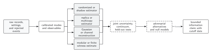
Raw field or simulator records pass through calibration, an estimator and model, correlated uncertainty, continuum checks, and adversarial alternatives before a bounded information claim is issued. — Entropy, tomography, witness, and recovery methods enter at the estimator stage, but all share calibration, uncertainty, continuum, and alternative-model tests. The final statement is no stronger than the least validated arrow. The diagram is schematic and not to scale.

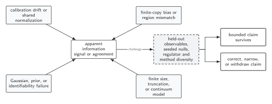
Calibration drift, finite copies, model mismatch, continuum extrapolation, and shared normalization can all imitate an information signal; held-out tests, method diversity, replication, and correction constrain them. — Different estimators can share the same calibration or normalization bias, so numerical agreement is not automatically independent replication. Adversarial nulls, held-out observables, regulator variation, and genuinely independent implementations set the claim ceiling and trigger correction when needed. The diagram is schematic.

References

Blanco, David D., Horacio Casini, Ling-Yan Hung, and Robert C. Myers. “Relative Entropy and Holography.” Journal of High Energy Physics 08 (2013): 060. DOI. Open PDF.
Lashkari, Nima, Michael B. McDermott, and Mark Van Raamsdonk. “Gravitational Dynamics from Entanglement ‘Thermodynamics’.” Journal of High Energy Physics 04 (2014): 195. DOI. Open PDF.