Interval, Sphere, and Cylinder Entanglement in CFT

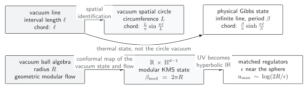
Intervals and balls are unusually tractable in a CFT because conformal maps turn their vacuum modular flow into a geometric flow. Three constructions must nevertheless remain distinct: a vacuum on a spatial circle, a physical Gibbs state obtained by compactifying Euclidean time, and the modular KMS representation of a vacuum ball on hyperbolic space. The continuum statement concerns local algebras and modular automorphisms. A literal reduced density matrix and von Neumann entropy appear only after a split/type-I replacement or UV regulator, whose cutoff surface must be transformed with the geometry. The resulting formulas are exact only for the mapped state and global identification.

Required background. Use Universal Terms and Entangling-Surface Geometry to distinguish an intrinsic universal coefficient from a regulated entropy. Helpful background. Replica and branched geometries supplies the twist-field path integral, including the conformal transformation law used for intervals.

Twist fields on the line, spatial cylinder, and Gibbs cylinder

Begin with a nonanomalous two-dimensional CFT and use the convention

$$c_L=c_R=c.$$

The branch-point twist field in the $n$-copy theory has

$$h_n=\bar h_n=\frac{c}{24}\left(n-\frac1n\right).$$

Let $\mathcal R$ denote a local UV regulator at both interval endpoints and let $\epsilon$ be its proper-distance cutoff. For $\epsilon\ll\ell$, the plane two-point function gives

$$S_n(\ell) =\frac{c}{6}\left(1+\frac1n\right)\log\frac{\ell}{\epsilon}+b_{n,\mathcal R}, \qquad S(\ell)=\lim_{n\to1}S_n(\ell) =\frac{c}{3}\log\frac{\ell}{\epsilon}+b_{1,\mathcal R}.$$

The constants $b_{n,\mathcal R}$ depend on the endpoint regulator and twist-field normalization; they are not universal CFT data. The derivation, including the twist-field weights, is given in Calabrese and Cardy 2004, §III.A, eqs. (10)–(19), pp. 8–10, PDF.

Now distinguish the two physical cylinders. For the vacuum on a spatial circle, let $w_c=\tau+ix$ with $x\sim x+L$ and use $z=\exp(2\pi w_c/L)$. Its interval must obey $0<\ell<L$ and $\epsilon\ll\min(\ell,L-\ell)$. For a Gibbs state on the infinite line, let $w_\beta=x+i\tau$ with $\tau\sim\tau+\beta$, $\beta>0$, and use $z=\exp(2\pi w_\beta/\beta)$; here $\epsilon\ll\min(\ell,\beta)$. Transforming the two twist insertions gives

$$S_{\rm circle}(\ell) =\frac{c}{3}\log\!\left[ \frac{L}{\pi\epsilon} \sin\!\left(\frac{\pi\ell}{L}\right) \right]+b_{1,\mathcal R},$$

and

$$S_{\rm thermal}(\ell) =\frac{c}{3}\log\!\left[ \frac{\beta}{\pi\epsilon} \sinh\!\left(\frac{\pi\ell}{\beta}\right) \right]+b_{1,\mathcal R}.$$

Writing the same $b_{1,\mathcal R}$ in both expressions is justified only when the same local endpoint scheme is transported through the conformal maps; independently chosen cutoffs can shift the two constants differently. The sine records a compact spatial direction and a pure vacuum; the hyperbolic sine records a compact Euclidean-time direction and a mixed physical Gibbs state. Neither is the modular KMS construction for a vacuum ball developed below. The formulas pass three immediate checks:

• both reduce to the line answer for $\ell\ll L,\beta$;
• the circle obeys $S(\ell)=S(L-\ell)$ by purity;
• for $\ell\gg\beta$, the thermal entropy becomes $\pi c\ell/(3\beta)+O(1)$, the extensive thermal entropy.

If the theory has a gravitational anomaly, do not silently reuse the symbol $c$. Fix the sign convention by ordering the endpoints and writing their Lorentzian separation as

$$\Delta x=\ell\cosh\varkappa, \qquad \Delta t=\ell\sinh\varkappa, \qquad \ell>0,$$

with the endpoint normal frames obtained by continuously boosting the equal-time laboratory frame. In this convention a rest-frame interval has coefficient $(c_L+c_R)/6$, while the boost contributes

$$S_{\rm boosted} =\frac{c_L+c_R}{6}\log\frac{\ell}{\epsilon} -\frac{c_L-c_R}{6}\varkappa+b_{1,\mathcal R}.$$

The second term depends on the normal-frame choice and changes sign when the ordered separation is boosted with $\varkappa\to-\varkappa$ Castro et al. 2014, §II.C.1–2, eqs. (2.19)–(2.24), pp. 7–9, PDF. It vanishes in the nonanomalous convention $c_L=c_R=c$ used above.

The chapter structure map places these results on the geometric branch. The canonical comparison table records why the vacuum circle, thermal line, and algebraic sharp-region statements have different domains.

The distinctions can be summarized before turning to the ball map:

Construction	State being represented	Diagnostic feature
Plane interval	Minkowski vacuum on an infinite line	Power-law twist correlator and $\log(\ell/\epsilon)$
Spatial cylinder	Pure vacuum on a circle of circumference $L$	Sine chord and $S(\ell)=S(L-\ell)$
Euclidean-time cylinder	Physical Gibbs state on an infinite line at inverse temperature $\beta$	Hyperbolic-sine chord and extensive large-$\ell$ entropy
Ball-to-hyperbolic map	Vacuum ball algebra represented as a KMS state for hyperbolic-time flow	Temperature $1/(2\pi R)$; not a thermal excitation of the original flat-space CFT

The figure shows the two physical interval cylinders and the distinct ball-to-hyperbolic-cylinder map. Inspect which cycle is compact in the interval panels and how the ball boundary is sent to the infinite end of hyperbolic space.

For the specified CFT vacuum or Gibbs state, exponential maps distinguish compact spatial and Euclidean-time cycles. Separately, the causal development of a vacuum ball maps to a modular KMS state on $\mathbb R\times\mathbb H^{d-1}$ at temperature $1/(2\pi R)$. The cutoff must be transformed with each map. Schematic; not to scale.

The vacuum ball and hyperbolic cylinder

Let $B$ be the ball $r<R$ at $t=0$ in Minkowski space. In $d=2$ spacetime dimensions, $B$ is the interval $(-R,R)$ and $\mathbb H^1$ is a noncompact line. Thus the construction below is also the vacuum-interval modular map in two dimensions; it is not the physical Gibbs state with inverse temperature $\beta$ from the preceding section. Coordinates $(\tau,u)$ on the causal development are related to Minkowski coordinates by

$$t=R\frac{\sinh(\tau/R)}{\cosh u+\cosh(\tau/R)}, \qquad r=R\frac{\sinh u}{\cosh u+\cosh(\tau/R)}.$$

The metric becomes

$$ds^2=\Omega^2\left[-d\tau^2+R^2\left(du^2+\sinh^2u\,d\Omega_{d-2}^2\right)\right], \qquad \Omega=\frac{1}{\cosh u+\cosh(\tau/R)}.$$

Thus the causal diamond is conformal to $\mathbb R\times\mathbb H^{d-1}$. Vacuum modular flow becomes translation in $\tau$, with temperature

$$T_0=\frac{1}{2\pi R}.$$

The map and temperature are derived in Casini, Huerta, and Myers 2011, §2.2, eqs. (2.25)–(2.31), pp. 11–13, PDF.

Intrinsically, the conformal transformation intertwines the ball algebra’s modular automorphism with hyperbolic-time evolution. A sharp continuum region need not possess a trace or density matrix Witten 2018, §§6.4–6.5, pp. 61–64. An exact density-matrix representation requires a type-I approximation whose cutoff surface, boundary conditions, and local counterterms are transported through the conformal map. For such a conformally matched regulator $\mathcal R$, one may write

$$U\rho_B^{\mathcal R}U^\dagger =\frac{e^{-2\pi R H_{\mathbb H}^{\mathcal R}}} {Z_{\mathbb H}^{\mathcal R}(2\pi R)},$$

with regulator-dependent boundary terms included on both sides. If the two cutoffs are imposed independently, this finite-regulator unitary identity need not hold, even though the continuum modular/KMS relation and properly matched universal terms do. In Minkowski variables the modular Hamiltonian is local,

$$K_B =2\pi\int_{r<R}d^{d-1}x\, \frac{R^2-r^2}{2R}T_{00}(x)+\text{constant}.$$

This is the push-forward of hyperbolic time translation Casini, Huerta, and Myers 2011, §2.1, eq. (2.20), p. 9, PDF. With the same cutoff prescription, the regulated entropy is the thermal entropy

$$S_B^{\mathcal R} =\left.(1-\beta\partial_\beta) \log Z_{\mathbb H}^{\mathcal R}(\beta)\right|_{\beta=2\pi R}.$$

At $\tau=0$, $r=R\tanh(u/2)$. If the flat-space cutoff removes $R-\epsilon<r<R$, then

$$e^{-u_{\max}}=\frac{\epsilon}{2R}+O(\epsilon^2/R^2),$$

so a UV cutoff near the sphere becomes an infrared volume cutoff on hyperbolic space Casini, Huerta, and Myers 2011, §2.2, eqs. (2.32)–(2.33), p. 13, PDF. In even $d$, including the Weyl anomaly yields the sphere logarithm

$$S_{B,\rm univ} =(-1)^{d/2-1}4A\log\frac{R}{\epsilon},$$

in the standard type-A anomaly normalization Casini, Huerta, and Myers 2011, §4.2, eq. (4.16), p. 29, PDF. In odd $d$ there is no local Weyl-anomaly logarithm; a round sphere instead has a real regulator-independent constant after local power-law divergences are removed. In $d=3$, define the real sphere free energy by $F=-\log\lvert Z(S^3)\rvert=-\operatorname{Re}\log Z(S^3)$. Then

$$S_{B,\rm univ}=\operatorname{Re}\log Z(S^3)=-F.$$

This equality uses the same regularization on the entropy and sphere-partition-function sides; taking the real part makes a possible partition-function phase irrelevant to this entropy constant Casini, Huerta, and Myers 2011, §5, eq. (5.1) and the following discussion, PDF. Omitting the cutoff transformation, the even-dimensional anomaly term, or the odd-dimensional constant breaks the corresponding map check.

These conformal identities are statements within QFT and do not require a holographic dual. For CFTs that do admit a controlled semiclassical AdS description, the Ryu–Takayanagi formula reproduces the interval and sphere results at leading holographic order under additional bulk assumptions; it does not define entanglement entropy for a generic CFT.

Mass and state failure tests

Consider a two-dimensional UV CFT with central charge $c$ deformed to a relativistic theory with a single controlling mass gap $m_{\rm gap}$ and correlation length $\xi=m_{\rm gap}^{-1}$. Assume a unique gapped vacuum, cluster decomposition, and no additional parametrically large correlation length. In the scaling window $\epsilon\ll\xi\ll\ell$, an interval with two endpoints has

$$S_{\rm massive}(\ell) =\frac{c}{3}\log\frac{\xi}{\epsilon}+O(1),$$

where each endpoint contributes $c\log(\xi/\epsilon)/6$ Calabrese and Cardy 2004, §IV.A, eq. (55) and the discussion after it, pp. 13–15, PDF. Here $c$ is the UV central charge. Multiple widely separated gaps, a degenerate vacuum, or gapless modes require a correspondingly richer crossover rather than this one-scale benchmark. The CFT formula would instead continue growing as $(c/3)\log(\ell/\epsilon)$. The scale-doubling diagnostic therefore makes the failure quantitative:

$$q(\ell)=\frac{S(2\ell)-S(\ell)}{\log2} \longrightarrow \begin{cases} c/3, & \ell\ll\xi,\\[2pt] 0, & \ell\gg\xi. \end{cases}$$

For $c=1$, extending the CFT growth from $\xi$ to $100\xi$ would add $(1/3)\log100\approx1.535$ even though the massive entropy has saturated, up to exponentially small corrections and constants. This is an order-one failure, not a shifted cutoff convention.

A generic excited state is a separate adversarial test. The spacetime conformal map still exists, but the state need not become the Gibbs state $e^{-2\pi R H_{\mathbb H}}/Z$. Infinitesimal state changes can be treated with the entanglement first law and the known $K_B$; a finite arbitrary excitation cannot be inserted into the vacuum thermal formula without mapping its preparation and operator insertions.

The validity map collects these failure modes together with spin structures, compact-space zero modes, anomaly conventions, and boundary conditions.

Common pitfalls

Interchanging the cylinder constructions. A spatial circle gives a sine and a pure-state complement relation. A Euclidean thermal circle gives a hyperbolic sine and extensive large-interval entropy. The ball-to-hyperbolic cylinder instead represents vacuum modular flow and is neither of those physical interval backgrounds.

Writing a sharp continuum density matrix as if it were intrinsic. State the algebraic modular-flow relation first. A density matrix formula requires a matched type-I regulator or split inclusion.

Keeping the same coordinate cutoff after a Weyl map. The sphere UV cutoff becomes a hyperbolic infrared cutoff. Transform it explicitly before comparing universal terms.

Exercises

1. Starting from the twist-field two-point function, derive the spatial-circle and physical Gibbs-cylinder replacements for the interval length.

Solution

A primary two-point function transforms with one factor of the map derivative at each endpoint. For $z=e^{2\pi w_c/L}$ with endpoints separated by $i\ell$, the derivative factors and $\lvert z_1-z_2\rvert$ combine into

$$\ell\longmapsto\frac{L}{\pi}\sin\frac{\pi\ell}{L}.$$

For $z=e^{2\pi w_\beta/\beta}$ with endpoints separated along the noncompact spatial direction, they combine into

$$\ell\longmapsto\frac{\beta}{\pi}\sinh\frac{\pi\ell}{\beta}.$$

Substituting these chord lengths into $S=(c/3)\log(\ell/\epsilon)+b_{1,\mathcal R}$ gives the two displayed formulas. The different analytic functions come from which coordinate is periodically identified.

2. At $\tau=0$, derive both the relation $r=R\tanh(u/2)$ and the leading cutoff map.

Solution

Setting $\tau=0$ in the coordinate map gives

$$r=R\frac{\sinh u}{\cosh u+1}=R\tanh\frac{u}{2}.$$

For large $u$, $\tanh(u/2)=1-2e^{-u}+O(e^{-2u})$. Therefore

$$R-r=2Re^{-u}+O(Re^{-2u}).$$

Putting $R-r=\epsilon$ at $u=u_{\max}$ yields $e^{-u_{\max}}=\epsilon/(2R)+O(\epsilon^2/R^2)$.

3. Let $c_L=2$, $c_R=1$, and use the ordered-endpoint convention above with $\varkappa=\log2$. Find the universal logarithmic coefficient and anomalous boost term.

Solution

The rest-frame coefficient is

$$\frac{c_L+c_R}{6}=\frac{3}{6}=\frac12.$$

The boost contribution is

$$-\frac{c_L-c_R}{6}\varkappa=-\frac{\log2}{6}.$$

Thus $S=(1/2)\log(\ell/\epsilon)-(\log2)/6+b_{1,\mathcal R}$. Reversing the boost reverses only the anomalous term.

4. For a massive theory with $\ell\gg\xi$, compare the scale-doubling estimator with the CFT prediction.

Solution

The massive entropy has saturated, so $S(2\ell)-S(\ell)\to0$ and $q(\ell)\to0$. The CFT formula gives

$$S_{\rm CFT}(2\ell)-S_{\rm CFT}(\ell) =\frac{c}{3}\log2,$$

hence $q_{\rm CFT}=c/3$. The disagreement in a difference eliminates the regulator-dependent additive constant, so it directly diagnoses the missing mass scale.

References

• Calabrese, Pasquale, and John Cardy. “Entanglement Entropy and Quantum Field Theory.” Journal of Statistical Mechanics: Theory and Experiment 2004, no. 06 (2004): P06002. DOI. Open PDF.
• Casini, Horacio, Marina Huerta, and Robert C. Myers. “Towards a Derivation of Holographic Entanglement Entropy.” Journal of High Energy Physics 2011, no. 05 (2011): 036. DOI. Open PDF.
• Castro, Alejandra, Stéphane Detournay, Nabil Iqbal, and Eric Perlmutter. “Holographic Entanglement Entropy and Gravitational Anomalies.” Journal of High Energy Physics 2014, no. 07 (2014): 114. DOI. Open PDF.
• Witten, Edward. “Notes on Some Entanglement Properties of Quantum Field Theory.” Reviews of Modern Physics 90, no. 4 (2018): 045003. DOI. Open PDF.