Entanglement Dynamics and Information Transport

Entanglement dynamics asks how quantum information becomes shared across space after a system is prepared away from equilibrium. The central lesson is that there is no single “information velocity.” Subregion entropy, mutual information, connected correlators, conserved charge, operator entanglement, and recovery performance are different observables. Quasiparticle, membrane, and hydrodynamic pictures can explain some of them in controlled regimes, but none may be substituted for the microscopic evolution or for the diagnostic that was actually measured.

Helpful background. Regulated subregion entropy supplies the continuum quantity, while mutual information supplies a finite correlation diagnostic. Equilibration and dephasing, OTOC regularization, and operator spreading distinguish neighboring dynamical questions. Real-time lattice evolution and quench regimes supply numerical and many-body baselines.

Enter this chapter

Begin with the state-preparation, quench, and regulator contract. It fixes the initial density operator, post-quench dynamics, physical region, subtraction, and order of limits. The next page extracts entanglement growth after quenches as direct data. Only then do the quasiparticle and membrane pages ask whether a simpler description predicts that data. Fronts, velocities, and bounds separates ballistic, diffusive, butterfly, causal, and entanglement scales.

The second sequence changes the diagnostic. Operator entanglement and channel–state maps turn a regulated evolution operator into a state-like object. Mutual information and correlator spreading compares an all-correlations quantity with operator-dependent two-point functions. Open and monitored dynamics separates conditioned trajectories from the unconditional density matrix. The final sequence studies conservation laws, integrable, chaotic, and localized dynamics, continuum finite-time windows, and a diagnostic comparison workflow.

The first diagram shows the logical order. Follow both arrows leaving the microscopic prediction: a direct diagnostic can be calculated even when no quasiparticle, membrane, or hydrodynamic reduction exists. An effective picture becomes useful only when it predicts a diagnostic that was not used to tune it.

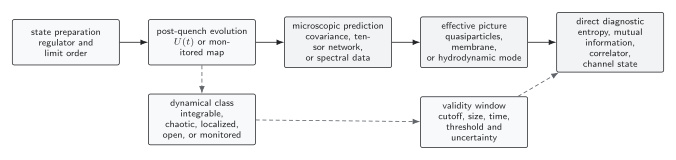
Direct observables follow from the regulated microscopic evolution whether or not an effective reduction is available. Quasiparticle, membrane, and hydrodynamic descriptions are explanatory layers that must predict those observables in a declared dynamical class and size–time window. The diagram is schematic and not to scale.

Direct observables and effective descriptions

For unitary evolution from a regulated state $\rho_0^{(a,L)}$,

$$\rho_A(t)=\operatorname{tr}_{\bar A} \!\left(U(t)\rho_0^{(a,L)}U(t)^\dagger\right), \qquad S_A(t)=-\operatorname{tr}\rho_A(t)\log\rho_A(t).$$

This equation defines a direct entropy calculation. A Gaussian covariance method, exact diagonalization, tensor network, or path integral may approximate it. By contrast, a formula involving entangled quasiparticle pairs or a minimizing membrane is an effective description. It has fewer inputs and therefore stronger predictive content, but also a narrower domain.

The distinction matters especially in continuum QFT. The bare entropy $S_A$ is cutoff dependent, so a calculation usually studies a common-cut subtraction such as

$$\Delta S_A(t)=S_A(t)-S_A(0),$$

or a regulator-compatible quantity such as mutual information for suitably separated regions or algebras. Even then, the state preparation can inject cutoff-scale energy. The continuum claim must keep physical masses, lengths, and observation times fixed while the regulator is refined. Cotler et al. 2016, §§ 2.1–2.4 and 3.1–3.3, pp. 9–24 provide a concrete free-scalar comparison of boundary-state and mass quenches, exact covariance entropies, and quasiparticle predictions.

An effective formula should be tested out of sample. For example, infer a membrane tension from one cut and predict another cut, or calculate the quasiparticle mode entropy and velocity from the quench and predict several interval lengths without an overall rescaling. Agreement obtained by refitting every geometry is a description of the data, not a successful dynamical law.

Growth laws require a declared window

After a homogeneous global quench, a finite interval often passes through four regimes:

1. a preparation-scale or regulator-scale transient;
2. an intermediate growth window;
3. a finite-region crossover or plateau;
4. a finite-volume return, recurrence, or numerical truncation regime.

In the boundary-state treatment of a one-dimensional conformal field theory, $\beta_{\rm eff}=4\tau_0$ relates the extrapolation length $\tau_0$ to an effective inverse temperature. For an interval of length $\ell$ at times and lengths large compared with $\tau_0$,

$$S_A(t)-S_A(0)\simeq \begin{cases} 2s_{\rm eq}t, & t<\ell/2,\\[2pt] s_{\rm eq}\ell, & t>\ell/2, \end{cases} \qquad s_{\rm eq}=\frac{\pi c}{3\beta_{\rm eff}}.$$

This is a scaling result, not a universal piecewise-linear law for every quench. The crossover is rounded at finite preparation scale; lattice dispersion, interactions, zero modes, inhomogeneity, and finite volume change the curve. The calculation of Calabrese and Cardy 2005, §§ 2–4 establishes the conformal baseline and its assumptions.

A commonly quoted chaotic-system fit,

$$\frac{dS_A}{dt}\simeq s_{\rm eq}v_E|\partial A|,$$

defines $v_E$ only after the boundary-area convention, entropy density, initial-state class, and fit window have been fixed. It does not by itself measure a signal velocity. Random circuits provide controlled models of minimal-cut growth and fluctuations Nahum et al. 2017, §§ II–IV, while Mezei and Stanford 2017, §§ 2–4 distinguish entanglement growth from an emergent information cone in chaotic systems.

Velocities answer different questions

Several quantities have dimensions of speed, but their definitions are not interchangeable:

• The relativistic causal speed bounds influence in a local continuum QFT.
• A Lieb–Robinson velocity bounds commutators in a specified lattice model; it is generally not the observed front speed.
• A group velocity $v_\alpha(k)=\partial_k\varepsilon_\alpha(k)$ transports a quasiparticle wave packet.
• A butterfly velocity is extracted from an operator-growth or OTOC front with a specified regularization and threshold.
• An entanglement velocity converts equilibrium entropy density and boundary area into a coarse-grained entropy-production rate.
• A diffusion constant $D$ has units of length squared per time. A threshold contour of a diffusive Gaussian grows as $\sqrt{Dt}$ and therefore has no constant asymptotic speed.

The inequality between any two of these depends on hypotheses and normalization. For example, chaotic locally equilibrating models often satisfy relationships between $v_E$ and an emergent butterfly or information-cone speed, but that does not make $v_E=v_B$ or turn a result in one model class into a theorem for all continuum QFTs. The fronts page develops operational extraction procedures and threshold tests.

Entanglement-dynamics diagnostic comparison

The table is a decision aid. Choose its first column before fitting a front or rate, then carry the remaining columns into the claim. The last column is deliberately adversarial: it names a change that can overturn an attractive interpretation.

Distinct information-dynamics diagnostics, their controlled regimes, and decisive comparisons

Diagnostic	Preparation and observable	Reported front or rate	Conservation input	Open-system assumption	Controlled limit	Required size–time window	Falsifying comparison
Subregion entropy	Pure or mixed quench; SA(t) or a common-cut subtraction	Initial curvature, growth slope, crossover, or plateau	Can alter leading behavior for inhomogeneous states and subleading behavior more generally	Unitary unless a channel and mixed-state diagnostic are declared	Exact covariance, tensor network, or controlled circuit	After the preparation transient and before truncation, saturation, or recurrence	Change region, cutoff, subtraction, and numerical bond dimension
Quasiparticle prediction	Mode-production entropy, species, and post-quench dispersion	Pair separation 2|vα(k)|t and entropy-weighted growth	Stationary occupations and dressed velocities in integrable models	Normally closed; scattering or loss needs a kinetic extension	Free or integrable space–time scaling limit	After pair production and before boundary return or strong inelastic scattering	Predict exact covariance data without refitting the mode entropy
Membrane law	Coarse-grained entropy profile and final entangling surface	Tension ℰ(v) and derived vE	Conserved hydrodynamic fields may couple to the entropy profile	Usually closed, chaotic, and locally equilibrated	Random circuit, holographic, or model-specific hydrodynamic scaling	Local-equilibration scale much smaller than region and observation scales	Fit one geometry and predict a distinct geometry
Connected correlator	Named local operators and a connected two-point function	Threshold arrival, peak, decay, and broadening	Strongly dependent on whether the operator overlaps a conserved mode	Heisenberg or channel evolution must be explicit	Free propagation, hydrodynamics, or converged numerics	Signal above the error floor and before reflection from boundaries	Choose an operator blind to the transported charge and vary the threshold
Mutual information	Two separated algebras, or reduced density matrices in a type-I regulator	Onset, peak, or decay of total correlations	Includes classical and quantum correlations in all retained sectors	Computed from the reduced state after the declared channel	Gaussian states, finite systems, or controlled replica calculations	Both regions resolved and regulator cancellation stable	Compare with several matched two-point functions
Operator entanglement	Normalized channel state for U(t) or a quantum channel	Growth across a specified input–output spatial partition	Symmetry blocks and reference measure must be retained	Unitary or channel normalization stated	Finite dimension or converged energy-constrained truncation	Cutoff converged at fixed reference energy, then reference profile varied	Identity and SWAP controls; change the channel-state reference
Monitored trajectory	Conditioned state and complete measurement record	Trajectory entropy growth or measurement-induced scaling	Symmetry of both unitary and measurement layers matters	Unraveling, efficiency, and postselection explicit	Hybrid circuits or specified continuously monitored models	Trajectory ensemble and finite-size scaling converged	Compare two unravelings of one unconditional master equation
Unconditional open-system state	Density operator averaged over unobserved outcomes	Mixing, decoherence, negativity, or recoverability rate	Bath may preserve or break the charge explicitly	Lindblad or microscopic environment model declared	Controlled weak-coupling, collision model, or finite simulation	Master-equation approximation and numerical truncation valid	Retain the record and compare average nonlinear diagnostics
Charge transport	Density profile, current, structure factor, or full counting statistics	Ballistic speed, diffusion constant, or anomalous exponent	Central defining input	Bath symmetry and continuity equation stated	Hydrodynamic or integrable scaling limit	After microscopic relaxation and before finite-volume return	Weakly break the conservation law and mix initial sectors
Recovery diagnostic	Encoding, noise channel, retained output, and recovery map	Fidelity, relative entropy loss, or recoverable information	Recovery may be sector constrained	Environment and accessible record are part of the task	Finite-dimensional code or energy-constrained channel	Optimization and truncation errors below the claimed effect	Entropy grows while an explicit recovery still succeeds

The table prevents a common category error. For a mixed state, $S_A$ is not an entanglement measure: local dephasing of a Bell pair leaves $S_A=\log 2$ even after the bipartite state becomes separable. Likewise, a connected correlator can vanish because the chosen operator is blind to a conserved mode, while mutual information remains nonzero. An operational conclusion should name the diagnostic that supports it rather than promoting “information” to an unspecified substance.

Failure controls that change the conclusion

Every dynamical claim should survive four independent families of changes.

Change the observable and extraction rule. Report the operator, region, Rényi index, threshold, fit norm, and uncertainty. A front that moves when the threshold is changed may be broadening rather than ballistic translation. A diffusive relative-threshold contour obeys $x_\theta(t)\propto\sqrt{t}$, so fitting it over a short interval to $vt$ produces a window-dependent “speed.”

Change the regulator and window. Refine the lattice at fixed physical geometry and time, reduce the timestep, increase the volume, and move the fit window. The desired regime should widen in physical units. A plateau that moves with bond dimension is truncation; a peak that moves with the boundary is reflection.

Change the dynamical class. Break integrability weakly, add or remove a conservation law, introduce disorder, or vary an inelastic scale. Integrable quasiparticle predictions, chaotic membrane laws, diffusive transport, and localized logarithmic growth are not interchangeable baselines. The same early-time curve may cross over to very different asymptotics.

Change what is observed about the environment. For monitored dynamics, compare the entropy or negativity of each conditioned trajectory with the corresponding quantity of the averaged density matrix. Because entropy and most entanglement measures are nonlinear, averaging states before evaluating the diagnostic does not equal averaging the diagnostic over trajectories. Measurement-induced transitions established in hybrid circuits concern trajectory ensembles with specified records and finite-size scaling; they are not generic theorems about every open continuum QFT Skinner, Ruhman, and Nahum 2019, §§ I–III.

Inspect the second diagram as a checklist: each lower box names the false conclusion produced by skipping the check directly above it.

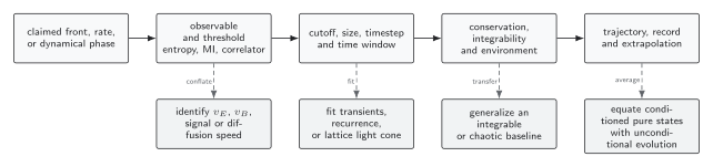
Observable choice, numerical window, dynamical class, and environmental record are logically independent controls. A claim that survives only one setting should be reported as a model- and protocol-specific observation, not as a universal information-transport law. The diagram is schematic.

Scope boundaries

This chapter treats entanglement and information diagnostics as outputs of nonequilibrium evolution. It uses, but does not redevelop, the microscopic theory of thermalization and quantum chaos, real-time contours, kinetic theory, hydrodynamics, or open QFT. It also does not use entropy growth as a proxy for the OTOC and operator-growth diagnostics that define scrambling more directly.

The final claim should therefore have the form: for this regulated preparation, this named observable exhibits this scaling over this converged window, and this effective description predicts it within these uncertainties. That sentence is longer than “information spreads ballistically,” but it is also scientifically useful.

Exercises

Take a $c=1$ conformal field theory with preparation scale $\tau_0=0.5$ and an interval of length $\ell=6$, using $\beta_{\rm eff}=4\tau_0$. Compute $s_{\rm eq}$, the early-time entropy slope, the scaling-limit saturation entropy, and the crossover time.

Solution

The effective inverse temperature is $\beta_{\rm eff}=2$, so

$$s_{\rm eq}=\frac{\pi}{3\beta_{\rm eff}}=\frac{\pi}{6}.$$

The early branch has slope $2s_{\rm eq}=\pi/3$. The plateau is $s_{\rm eq}\ell=\pi$, and the scaling crossover occurs at $t=\ell/2=3$. These are the values of the idealized conformal scaling form; a regulated calculation should show rounded crossovers.

A one-dimensional diffusive density has

$$n(x,t)=\frac{1}{\sqrt{4\pi Dt}}e^{-x^2/(4Dt)}.$$

Define a front by $n(x_\theta,t)/n(0,t)=\theta$ with $0<\theta<1$. Find $x_\theta(t)$ and compare its value at $4t$ with its value at $t$. Why is a constant fitted speed misleading?

Solution

The ratio cancels the time-dependent amplitude:

$$e^{-x_\theta^2/(4Dt)}=\theta, \qquad x_\theta(t)=2\sqrt{Dt\log(1/\theta)}.$$

Therefore $x_\theta(4t)=2x_\theta(t)$. The instantaneous ratio $x_\theta/t$ decays as $t^{-1/2}$, so a linear fit returns a number that depends on the chosen window rather than an asymptotic velocity.

A Bell state $|\Phi^+\rangle=(|00\rangle+|11\rangle)/\sqrt2$ is completely dephased in the computational basis. Compare the mutual information before and after dephasing, and explain why the subsystem entropy alone does not diagnose the loss of entanglement.

Solution

Initially the joint state is pure and each qubit is maximally mixed, so

$$I(A:B)=S_A+S_B-S_{AB}=2\log2.$$

Complete dephasing gives

$$\rho_{AB}=\frac12|00\rangle\langle00|+\frac12|11\rangle\langle11|.$$

Now $S_A=S_B=S_{AB}=\log2$, so $I(A:B)=\log2$. The remaining correlations are classical and the state is separable, but $S_A$ stayed equal to $\log2$. For mixed states, subsystem entropy includes both entanglement and classical or environmental mixing; use a mixed-state entanglement measure or an operational task.

References

• Alba, Vincenzo, and Pasquale Calabrese. “Entanglement and Thermodynamics after a Quantum Quench in Integrable Systems.” Proceedings of the National Academy of Sciences 114 (2017): 7947–7951. DOI.
• Calabrese, Pasquale, and John Cardy. “Evolution of Entanglement Entropy in One-Dimensional Systems.” Journal of Statistical Mechanics: Theory and Experiment 2005 (2005): P04010. DOI.
• Cotler, Jordan S., Mark P. Hertzberg, Márk Mezei, and Mark T. Mueller. “Entanglement Growth after a Global Quench in Free Scalar Field Theory.” Journal of High Energy Physics 2016, no. 11 (2016): 166. DOI.
• Mezei, Márk, and Douglas Stanford. “On Entanglement Spreading in Chaotic Systems.” Journal of High Energy Physics 2017, no. 5 (2017): 065. DOI.
• Nahum, Adam, Jonathan Ruhman, Sagar Vijay, and Jeongwan Haah. “Quantum Entanglement Growth under Random Unitary Dynamics.” Physical Review X 7 (2017): 031016. DOI.
• Skinner, Brian, Jonathan Ruhman, and Adam Nahum. “Measurement-Induced Phase Transitions in the Dynamics of Entanglement.” Physical Review X 9 (2019): 031009. DOI.