Cost Geometry, Gate Sets, and Reference States

Nielsen geometry replaces a discrete circuit search by a variational problem on a Lie group of regulated transformations. The method becomes a complexity definition only after the generators, their normalization, the invariant convention, the cost function, the reference and target, and the global minimization rule are fixed. A geodesic is a candidate path; it is not automatically the least-cost circuit.

Required background. Direct Sums, Tensor Products, and Index Structure supplies the composite regulated space and generator basis. Circuit Complexity in Quantum Field Theory supplies the approximation task that the continuous geometry models.

Paths, generators, and invariant costs

Let $U(s)$, $0\leq s\leq1$, connect $U(0)=\mathbb 1$ to a representative of the target. In a right-invariant convention,

$$\dot U(s)=-iY^I(s)M_IU(s), \qquad Y^I(s)M_I=i\dot U(s)U(s)^{-1}.$$

A local cost $F(U,Y)$ defines the path length

$$L[U]=\int_0^1F(U(s),Y(s))\,ds, \qquad C(U_{\rm tar})=\inf_{U(1)\sim U_{\rm tar}}L[U].$$

The equivalence $\sim$ must be stated. For state preparation, $U(1)$ may be multiplied by any stabilizer of the reference or target that leaves the prepared state unchanged. For unitary synthesis the quotient is usually smaller. Left-invariant coordinates instead use $iU^{-1}\dot U$; changing convention without translating penalties changes the geometry. The differential-geometric relation between these choices and quantum circuits is developed by Dowling and Nielsen 2008, §§II–IV.

Common homogeneous costs include

$$F_1(Y)=\sum_I p_I\lvert Y^I\rvert, \qquad F_2(Y)=\left(\sum_I p_I(Y^I)^2\right)^{1/2}.$$

The weights $p_I>0$ penalize selected directions. Homogeneity makes length invariant under monotone reparameterization, so path parameter is not physical time. Generator normalization matters: replacing $M_I$ by $\alpha_I M_I$ requires $Y^I\to Y^I/\alpha_I$ and a compensating penalty translation if the same physical cost is intended.

Geodesic equations and what they prove

For a quadratic right-invariant metric $G_{IJ}$, extremizing the energy $E=\tfrac12\int ds\,G_{IJ}Y^IY^J$ gives the Euler–Arnold equation

$$\dot\Pi_K=f_{KI}{}^{J}Y^I\Pi_J, \qquad \Pi_I=G_{IJ}Y^J,$$

with structure constants $[M_I,M_J]=if_{IJ}{}^KM_K$. Solving this boundary-value problem finds stationary paths. Three further checks are required:

1. the endpoint satisfies the target equivalence and approximation tolerance;
2. the second variation has no negative direction before the endpoint, or conjugate points are treated;
3. competing homotopy classes and nonsmooth $F_1$ paths have been searched well enough to support global minimality.

Nielsen’s geometric construction was introduced as a route to circuit lower bounds under explicit penalty schedules Nielsen 2006, §§2–4. It does not select a unique metric for QFT.

One-mode squeeze under two metrics

For a single Gaussian mode, take a squeeze generator $M_s$ and target parameter $r$. The path $U(s)=e^{-isrM_s}$ has $Y^s=r$. With $p_s=1$, both $F_1$ and $F_2$ give $|r|$ because the tangent space is one-dimensional.

For $N$ independent modes with coordinates $r_k$, the same straight path gives

$$C_1=\sum_{k=1}^N\lvert r_k\rvert, \qquad C_2=\left(\sum_{k=1}^Nr_k^2\right)^{1/2}.$$

If $r_k=r$, the ratio $C_1/C_2=\sqrt N$ grows with the regulator dimension. Finite-dimensional norm equivalence therefore does not establish continuum equivalence. Penalties for entangling or nonlocal gates can alter both the path and its ultraviolet scaling.

Practical minimization workflow

1. Choose a finite regulator and an orthonormal generator convention.
2. State the quotient by stabilizers and the endpoint error metric.
3. Evaluate an explicit admissible path to obtain an upper bound.
4. Solve the geodesic or optimal-control equations and retain all candidate branches.
5. Test conjugate points, branch crossings, and shorter composite paths.
6. repeat under a second penalty schedule and finer regulator at fixed physical accuracy.

Numerical shooting should report endpoint residual, conserved quantities, discretization convergence, and sensitivity to initial seeds. A solver returning one smooth curve is not evidence of the global infimum.

Common pitfalls

Calling the metric canonical. Symmetry can restrict a cost, but it rarely fixes every penalty or normalization. State the residual family and which conclusion is stable across it.

Calling length duration. A homogeneous path length is invariant under reparameterization. Physical duration appears only after control amplitudes and an implementation Hamiltonian are bounded.

Exercises

Generator rescaling. Let $M'=2M$ and $U=e^{-irM}$. What coefficient represents the same path, and what happens if the penalty is not translated?

Solution

The coefficient is $r'=r/2$. With an unaltered unit penalty, the numerical length is halved even though the transformation is identical. The cost convention, not the physics, changed.

Local versus global. Why does a positive second variation along one geodesic not prove it is the complexity?

Solution

It proves only local minimality up to the tested endpoint and variations. A distinct geodesic, another stabilizer representative, a different homotopy class, or a nonsmooth path can have smaller length. Global comparison is a separate step.

Task and validity maps

The first diagram distinguishes target objects and their admissible resource models; inspect which equivalence class is being minimized over. The second shows the definition changes and physical controls that must be held fixed before two complexity values or growth laws are compared.

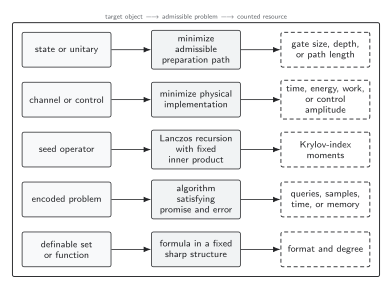
A complexity value is defined only after the target object selects an admissible family of paths or descriptions. Circuit length, physical control cost, Krylov spread, algorithmic resources, and sharp o-minimal format or degree answer different questions. The diagram is schematic and not to scale.

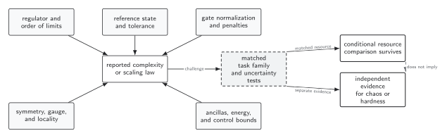
Reference sensitivity, gate nonuniqueness, regulator dependence, symmetry constraints, and unbounded controls are distinct failure modes. A link from complexity growth to chaos or computational hardness requires separate evidence after those controls. The diagram is schematic.

References

• Dowling, Mark R., and Michael A. Nielsen. “The Geometry of Quantum Computation.” Quantum Information & Computation 8 (2008): 861–899. Open PDF.
• Nielsen, Michael A. “A Geometric Approach to Quantum Circuit Lower Bounds.” Quantum Information & Computation 6 (2006): 213–262. Open PDF.