Complex Saddles, Lefschetz Thimbles, and Integration Cycles

A complex critical point contributes only when its steepest-descent cycle occurs in the homology class of the original integration cycle. The coefficients are oriented intersection numbers with dual cycles, and the Gaussian phases follow from the orientation and Hessian branch on each thimble. Complexifying the field equations is therefore necessary but not sufficient.

Required background. Laplace’s method and steepest descent supplies convergent contour deformation in a regulated integral; negative modes and instability indices supplies the relation between local Gaussian directions and contour phases.

Helpful background. Stationary phase, coalescing saddles, and Stokes phenomena supplies uniform finite-dimensional asymptotics; Wick rotation and analytic continuation supplies the distinction between an analytic continuation and an assumed Euclidean contour.

Downward cycles and their duals

Begin with a finite-dimensional regulator,

$$Z_\Gamma(g)=\int_\Gamma \Omega(z)\, \exp[-h(z;g)], \qquad h(z;g)=\frac{S(z;g)}{\epsilon},$$

where $S$ is holomorphic, $\Omega$ is a holomorphic top form, and $\Gamma$ is a convergent middle-dimensional cycle in the complexified configuration space. Suppose the critical points $z_\sigma$ are isolated and nondegenerate.

Choose a Hermitian metric $G_{i\bar j}$ and define the upward-$\operatorname{Re}h$ flow

$$\frac{dz^i}{dt} =G^{i\bar j}\, \overline{\frac{\partial h}{\partial z^j}}.$$

Along it,

$$\frac{d}{dt}\operatorname{Re}h =G^{i\bar j} \frac{\partial h}{\partial z^i} \overline{\frac{\partial h}{\partial z^j}} \geq0, \qquad \frac{d}{dt}\operatorname{Im}h=0.$$

The downward integration cycle $\mathcal J_\sigma$ consists of trajectories approaching $z_\sigma$ as $t\to-\infty$ and running toward regions with $\operatorname{Re}h\to+\infty$. The dual cycle $\mathcal K_\sigma$ is defined by the opposite flow. With compatible orientations,

$$\langle\mathcal J_\sigma,\mathcal K_\tau\rangle =\delta_{\sigma\tau}, \qquad \Gamma=\sum_\sigma n_\sigma\mathcal J_\sigma, \qquad n_\sigma=\langle\Gamma,\mathcal K_\sigma\rangle\in\mathbb Z.$$

This answers the coefficient question: $n_\sigma$ is fixed by the original cycle, not by comparing critical values. The local contribution is

$$Z_\sigma \sim e^{-h_\sigma} \frac{(2\pi)^{N/2}\,\Omega(z_\sigma)} {\sqrt{\det H_\sigma}}\, \bigl[1+O(\epsilon)\bigr], \qquad (H_\sigma)_{ij} =\frac{\partial^2 h}{\partial z^i\partial z^j}\bigg|_{z_\sigma}.$$

The square-root branch is continued along the oriented thimble. Choosing a principal square root independently at each saddle generally gives inconsistent phases. Witten 2011, §§2.1–3.1, preprint pp. 5–23 develops the relative-homology construction and its intersection pairing.

The construction requires modification at a degenerate critical point, at a singularity of $\Omega$, or when flow escapes to a nonconvergent end. In a gauge theory, gauge fixing or an appropriate quotient is required before the critical set can be treated as Morse. In continuum QFT, a lattice, mode cutoff, or other regulator must define both the complexified space and the cycle before formal infinite-dimensional flow equations acquire mathematical meaning.

A quartic integral

Consider the normalized zero-dimensional quartic integral

$$Z(g)=\frac1{\sqrt{2\pi}} \int_{\mathbb R}\mathrm dx\, \exp\!\left(-\frac{x^2}{2}-\frac{g x^4}{4}\right), \qquad \operatorname{Re}g>0.$$

The critical points of

$$S(z;g)=\frac{z^2}{2}+\frac{g z^4}{4}$$

are

$$z_0=0, \qquad z_\pm=\pm\frac{i}{\sqrt g},$$

with critical values

$$S_0=0, \qquad S_\pm=-\frac1{4g}.$$

All three saddles exist for $g\neq0$, but on the positive real contour only the thimble content selected by $\mathbb R$ contributes. In particular, the exponentially large factors $e^{+1/(4g)}$ associated with $z_\pm$ for $g>0$ do not appear merely because those critical points exist.

The integral can be evaluated exactly:

$$Z(g) =\frac{e^{1/(8g)}}{2\sqrt{\pi g}}\, K_{1/4}\!\left(\frac1{8g}\right), \qquad \operatorname{Re}g>0,$$

with branches fixed by continuation from positive $g$. The formula follows from the real integral representation of the modified Bessel function; see NIST DLMF, §10.32(i), Eq. 10.32.9. Its small-$g$ asymptotic expansion begins with $Z(g)\sim1-3g/4+\cdots$, while the other critical values set the exponential scales that can enter after analytic continuation.

Write $g=\rho e^{i\theta}$ with $\rho>0$, and denote the lower and upper lateral limits by

$$X^-=X(\theta=-\delta), \qquad X^+=X(\theta=+\delta), \qquad 0<\delta\ll1.$$

The positive real axis is a Stokes wall because $\operatorname{Im}(S_\pm-S_0)=0$. At $\theta=0$, use the flat metric and put $z=iy$ in the upward flow. It reduces to

$$\dot y=y(\rho y^2-1).$$

For $0<|y|<1/\sqrt\rho$, the two oriented trajectories run from $z_+$ and $z_-$ toward $z_0$. There is no nonconstant $z_+\leftrightarrow z_-$ connection: their critical values agree, whereas $\operatorname{Re}S$ strictly increases along every nonconstant upward trajectory.

The four convergence-wedge centers are

$$\alpha_k(\theta) =-\frac{\theta}{4}+\frac{k\pi}{2}, \qquad k=0,1,2,3,$$

and will be called $A,B,C,D$ in that order. Orient the complex plane by $dx\wedge dy$, the continued real cycle from left to right, $\mathcal J_0$ locally along $+1$, $\mathcal J_\pm$ locally along $+i$, $\mathcal K_0$ locally along $+i$, and $\mathcal K_\pm$ locally along $-1$. These choices fix the signs below, rather than merely the absolute incidence of the flows.

The figure shows the upper-lateral geometry at $g=e^{0.15i}$ and the actual lower-to-upper Stokes transformation. The drawn curves are schematic, but their endpoint sectors, local tangents, intersections, and orientations were checked from the flow.

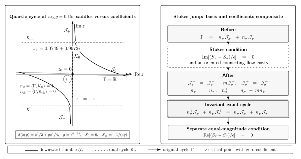
Schematic thimble map for the regulated quartic integral, not to scale. The left panel is the upper-lateral geometry at $g=e^{0.15i}$; the right panel follows the lower-to-upper crossing through $\arg g=0$. With the printed orientations, both complex thimbles jump with $m_+=m_-=-1$, while the real contour stays $\Gamma=\mathcal J_0$ and its coefficient vector remains $(1,0,0)$.

The signed quartic Stokes jump

The oriented endpoint chains on the two sides are

Lateral side	$\mathcal J_0$	$\mathcal J_+$	$\mathcal J_-$
$\theta=-\delta$	$C\to A$	$C\to B$	$D\to A$
$\theta=+\delta$	$C\to A$	$A\to B$	$D\to C$

Composition of oriented paths gives

$$C\to B=(C\to A)+(A\to B), \qquad D\to A=(D\to C)+(C\to A).$$

Therefore the lower-to-upper basis transformation is

$$\boxed{\mathcal J_0^+=\mathcal J_0^-}, \qquad \boxed{\mathcal J_\pm^+ =\mathcal J_\pm^- -\mathcal J_0^-}.$$

Thus the two signed Picard–Lefschetz integers are $m_+=m_-=-1$ in the convention $\mathcal J_\tau^+=\mathcal J_\tau^-+m_\tau\mathcal J_0^-$. Reversing the crossing reverses both signs. In the ordered basis $(0,+,-)$,

$$\begin{pmatrix} \mathcal J_0^+\\ \mathcal J_+^+\\ \mathcal J_-^+ \end{pmatrix} = \begin{pmatrix} 1&0&0\\ -1&1&0\\ -1&0&1 \end{pmatrix} \begin{pmatrix} \mathcal J_0^-\\ \mathcal J_+^-\\ \mathcal J_-^- \end{pmatrix}.$$

The dual basis and coefficients transform inversely:

$$\mathcal K_0^+ =\mathcal K_0^-+\mathcal K_+^-+\mathcal K_-^-, \qquad \mathcal K_\pm^+=\mathcal K_\pm^-,$$ $$n_0^+=n_0^-+n_+^-+n_-^-, \qquad n_\pm^+=n_\pm^-.$$

For the continued real contour, $\Gamma$ and $\mathcal J_0$ both represent $C\to A$. Hence

$$(n_0,n_+,n_-)^-=(n_0,n_+,n_-)^+=(1,0,0), \qquad \Gamma=\mathcal J_0^- =\mathcal J_0^+.$$

The complex basis elements jump even though their coefficients in this particular physical cycle vanish on both sides. For another cycle with $n_\pm\neq0$, the displayed inverse transformation changes $n_0$ so that the exact cycle remains invariant. The signed calculation—not a drawing alone—determines this cancellation, and the Bessel representation supplies an independent check of the same lateral continuation.

It is useful to distinguish two conditions:

$$\begin{aligned} \text{phase alignment:}\quad& \operatorname{Im}\frac{S_\sigma-S_\tau}{\epsilon}=0,\\ \text{equal exponential magnitude:}\quad& \operatorname{Re}\frac{S_\sigma-S_\tau}{\epsilon}=0. \end{aligned}$$

This chapter calls the first condition a Stokes condition when a connecting flow exists, and the second an anti-Stokes condition. Some literature exchanges the names; the equations remove the ambiguity.

Boundaries of the method

A complex saddle calculation is controlled only when:

• the original Lorentzian or Euclidean prescription defines $\Gamma$;
• the regulator preserves the analytic structure needed for contour deformation;
• all singularities crossed by the deformation are included;
• critical points and flows are isolated or treated by a valid Morse–Bott generalization;
• the regulator can be removed without losing convergence or changing the claimed observable.

Real-time QFT, gauge orbit spaces, fermion determinants with zeros, and infinite-volume limits can violate several conditions at once. Formal complex solutions are still useful candidates, but their contribution and phase remain unproved until a cycle or an equivalent analytic-continuation prescription is supplied. Alexandru et al. 2022, §§II–III reviews how finite regulators, residual phases, multimodality, and continuum limits enter modern thimble algorithms.

Shared comparison. The canonical saddle comparison places this contour requirement beside the action, spectrum, determinant, renormalization, and breakdown data required of any saddle calculation.

Common pitfalls

Counting every complex solution. Existence solves only the critical-point equation. The intersection number with the original cycle can vanish.

Assigning Gaussian phases by a principal square root. The correct branch is transported continuously with the oriented thimble. Independent local branch choices can violate analyticity.

Calling every phase-alignment ray a jump. A Stokes jump also requires a connecting flow with nonzero incidence. Global topology can make the jump coefficient zero.

Exercises

1. Verify the critical points and critical values of the quartic integral.

Solution

Since

$$S'(z)=z+gz^3=z(1+gz^2),$$

the critical points are $z_0=0$ and $z_\pm=\pm i/\sqrt g$. At $z_\pm$, $z^2=-1/g$ and $z^4=1/g^2$, so

$$S(z_\pm)=-\frac1{2g}+\frac1{4g} =-\frac1{4g}.$$

2. Prove that $\operatorname{Im}h$ is constant along the thimble flow.

Solution

Using $\dot z^i=G^{i\bar j}\overline{\partial_j h}$,

$$\frac{dh}{dt} =G^{i\bar j}\partial_i h\,\overline{\partial_j h},$$

which is real and nonnegative because $G$ is Hermitian and positive definite. Hence the imaginary part is constant and the real part increases away from the saddle. The displayed flat-metric formula is recovered when $G_{i\bar j}=\delta_{ij}$.

3. Using the oriented endpoint sectors $A,B,C,D$, derive the two signed quartic Stokes jumps and show that the real contour has the same intersection numbers on both lateral sides.

Solution

On the lower lateral side,

$$\mathcal J_0^-=C\to A, \qquad \mathcal J_+^-=C\to B, \qquad \mathcal J_-^-=D\to A.$$

On the upper lateral side,

$$\mathcal J_0^+=C\to A, \qquad \mathcal J_+^+=A\to B, \qquad \mathcal J_-^+=D\to C.$$

Composition of oriented paths gives

$$C\to B=(C\to A)+(A\to B), \qquad D\to A=(D\to C)+(C\to A).$$

Therefore $\mathcal J_\pm^+=\mathcal J_\pm^- -\mathcal J_0^-$, so $m_+=m_-=-1$ for the stated orientations. Since $\Gamma=C\to A=\mathcal J_0^\pm$,

$$(n_0,n_+,n_-)^-=(n_0,n_+,n_-)^+=(1,0,0).$$

Continue from thimbles to parameter-dependent asymptotics

• To decide what changes on Stokes and equal-magnitude loci while the exact cycle remains fixed, continue to Stokes Jumps, Saddle Dominance, and Contour Dependence.
• For the finite-dimensional geometry underlying downward cycles and their intersections, return to Laplace’s method and steepest descent; for rigorous infinite-dimensional status, use Volume 16: Mathematical QFT and Rigorous Structures.
• To connect thimble jumps with lateral resummation and ambiguity cancellation, continue to Resurgence, Transseries, and Large-Order Structure.

References

• Alexandru, Andrei, Gökçe Başar, Paulo F. Bedaque, and Neill C. Warrington. “Complex Paths Around the Sign Problem.” Reviews of Modern Physics 94 (2022): 015006. arXiv:2007.05436. DOI.
• Olver, Frank W. J., et al., eds. NIST Digital Library of Mathematical Functions, §10.32, “Integral Representations” for modified Bessel functions. National Institute of Standards and Technology. DLMF.
• Witten, Edward. “Analytic Continuation of Chern–Simons Theory.” In Chern–Simons Gauge Theory: 20 Years After, AMS/IP Studies in Advanced Mathematics 50 (2011): 347–446. arXiv:1001.2933.