The CP(N-1) Model

The $\mathrm{CP}^{N-1}$ model turns a constrained complex vector into a projective field by identifying its local phase. That redundancy produces a composite $U(1)$ connection, quantized flux on suitable closed Euclidean spacetimes, and a theta angle. At large $N$ the connection and the constraint multiplier become useful independent integration variables, but their saddle parameters must still be translated into gauge-invariant observables. Claims about the phase at $\theta=\pi$ depend on $N$, global structure, boundary conditions, and the controlled regime.

Required background. Sigma-model target geometry and control supplies the quotient construction, while gauge fields, redundancy, and observables distinguishes a redundant phase from a physical symmetry. Helpful background. Theta terms and vacuum sectors fixes the general periodicity question, and large-N normalizations fixes the order of limits.

Projective field and emergent connection

Let

$$z(x)\in\mathbb C^N,\qquad z^\dagger z=1,$$

with the local equivalence

$$z(x)\sim e^{i\alpha(x)}z(x).$$

The physical field is the rank-one projector

$$P=zz^\dagger,\qquad P^2=P,\qquad \operatorname{tr}P=1,$$

which is invariant under the redundant phase. Define

$$A_\mu=-i\,z^\dagger\partial_\mu z, \qquad D_\mu z=(\partial_\mu-iA_\mu)z .$$

Then $A_\mu\mapsto A_\mu+\partial_\mu\alpha$ and $D_\mu z\mapsto e^{i\alpha}D_\mu z$. The two-derivative Euclidean action is

$$S_E =\frac{1}{g_0^2} \int\mathrm d^2x\, (D_\mu z)^\dagger D_\mu z +i\theta Q .$$

The overall factor is a convention; here it is chosen so that the large-$N$ gap equation below has the same integral normalization as the chapter’s $O(N)$ example. The faithful continuous global symmetry acting on local gauge-invariant fields is $PSU(N)=SU(N)/\mathbb Z_N$, not an extra copy of the redundant $U(1)$.

Varying the action with respect to an independent algebraic $A_\mu$ gives

$$A_\mu=-i\,z^\dagger\partial_\mu z,$$

so the gauge-like presentation is exactly equivalent to the projective kinetic term at this classical level. Quantum mechanically it is often more useful to integrate over $A_\mu$ and impose the constraint with a multiplier. A Maxwell term is then generated by matter fluctuations even though none was present in the original two-derivative action.

Flux and topological charge

The curvature of the composite connection is

$$F_{\mu\nu} =\partial_\mu A_\nu-\partial_\nu A_\mu =-i\left[ (\partial_\mu z)^\dagger\partial_\nu z -(\partial_\nu z)^\dagger\partial_\mu z \right].$$

On an oriented closed Euclidean two-manifold with no nontrivial background $PSU(N)$ bundle, when the projective field defines an ordinary smooth line bundle and the gauge transformations have the standard $U(1)$ periods,

$$Q =\frac{1}{2\pi}\int F \in\mathbb Z.$$

Therefore $e^{-i\theta Q}$ in the ordinary-background Euclidean path-integral weight is $2\pi$-periodic in $\theta$. This statement has two important global qualifications. On a manifold with boundary, the bulk integral need not be an integer by itself; boundary conditions, edge degrees of freedom, or a boundary counterterm must be specified. In a non-liftable background $PSU(N)$ bundle $E$, the $U(1)$ flux is correlated with the obstruction class $w_2(E)\in H^2(M,\mathbb Z_N)$. Then $\theta\mapsto\theta+2\pi$ shifts a quantized background counterterm rather than leaving $Z[\theta,E]$ pointwise unchanged. Center-twisted compactifications can likewise contain semiclassical events of charge $1/N$, even though the ordinary-background partition function retains its $2\pi$ period. The background-bundle statement and its anomaly consequence are derived in Gaiotto et al. 2017, § 1.1, pp. 3–5.

For $N=2$, $\mathrm{CP}^1\simeq S^2$, and the charge agrees with the degree of the corresponding $O(3)$ sigma-model map after matching orientations and action normalizations. This special equivalence should not be extrapolated to arbitrary $N$.

Large-N auxiliary saddle

Set $t_0=Ng_0^2$ and rescale $w=z/g_0$, so $w^\dagger w=N/t_0$. A useful regulated action is

$$S_E[w,A,\lambda] =\int\mathrm d^2x\, \left[ \lvert D_\mu w\rvert^2 +\lambda\left( w^\dagger w-\frac{N}{t_0} \right) \right] +i\theta Q .$$

Choosing the multiplier contour through a real positive saddle and integrating the $N$ complex components gives, at $\theta=0$,

$$\frac{S_{\mathrm{eff}}[A,\lambda]}{N} =\operatorname{Tr}\ln(-D^2+\lambda) -\frac{1}{t_0}\int\mathrm d^2x\,\lambda .$$

The translation-invariant saddle $A_\mu=0$, $\lambda=m^2>0$ obeys

$$\frac{1}{t_0} =\int_{\lvert p\rvert<\Lambda} \frac{\mathrm d^2p}{(2\pi)^2} \frac{1}{p^2+m^2} =\frac{1}{4\pi} \ln\!\left(1+\frac{\Lambda^2}{m^2}\right).$$

Remove the cutoff at fixed

$$\frac{1}{t_R(\mu)} =\frac{1}{t_0} -\frac{1}{4\pi}\ln\!\frac{\Lambda^2}{\mu^2}.$$

At leading $N=\infty$ this gives

$$\mu\frac{\mathrm dt_R}{\mathrm d\mu} =-\frac{t_R^2}{2\pi}, \qquad m=\mu\exp\!\left[-\frac{2\pi}{t_R(\mu)}\right].$$

Thus the large-$N$ saddle is asymptotically free and replaces a dimensionless coupling by an RG-invariant scale. Finite-$N$ corrections begin beyond this leading saddle and depend on the coupling convention. The derivation and its normalization are reviewed in Mariño 2015, § 6.3, pp. 201–215, while the large-$N$ theta branches are developed in Witten 1979, §§ 2–3. The scale and projector round trips are reproduced in the chapter’s benchmark.

It is not automatically the pole mass of a physical $z$ particle. The field $z$ is gauge-charged under the redundant $U(1)$ and cannot create an isolated gauge-invariant asymptotic state. The saddle controls a gauge-dependent inverse range in the charged propagator after gauge fixing and the threshold entering the induced effective action. Physical masses must be extracted from gauge-invariant operators such as

$$\mathcal O^A=z^\dagger T^A z$$

or from finite-volume energy levels. At leading large $N$, integrating out $w$ also generates a Maxwell term for $A_\mu$; its long-distance dynamics and the constraint field reorganize the gauge-invariant spectrum.

Dual variables and their conditions

The figure collects three transformations used in this chapter. None is an unconditional identification of elementary particles: every arrow carries a constraint, measure, anomaly, or boundary condition, and the round trip is checked on observables.

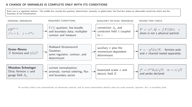
Dual and auxiliary variables expose otherwise hidden dynamics, but they do not erase the definition of the theory. In $\mathrm{CP}^{N-1}$ the $U(1)$ quotient and bundle data accompany the connection; in Gross–Neveu the Hubbard–Stratonovich field is fixed by its equation of motion and determinant; in the Schwinger model the current normalization, anomaly, flux sector, and external-probe definition accompany bosonization. The diagram is schematic rather than a spectrum plot.

The model’s position relative to the other strong-coupling examples is summarized by the laboratory map and its regime table.

Theta claims require a regime

Three statements are often conflated:

• Exact kinematics: integer $Q$ under the stated global conditions implies $2\pi$ periodicity of the partition function.
• Large N: the vacuum energy is organized into branches whose envelope restores $2\pi$ periodicity; a branch crossing can occur at $\theta=\pi$.
• Semiclassics: on a specified weakly coupled compactification, dilute integer or fractional events can generate a calculable theta-dependent potential.

Agreement of periodicity and anomalies is a cross-check, but the functional form of the vacuum energy and the infrared phase are dynamical. In particular, the familiar gapless $\theta=\pi$ behavior of $\mathrm{CP}^1\simeq O(3)$ is not a universal result for every $\mathrm{CP}^{N-1}$ model. The detailed separation is developed in Theta Terms and Topological Effects in Sigma Models.

Common pitfalls

Treating A as a new microscopic photon. In the minimal projective action, $A_\mu$ begins as an algebraic composite or auxiliary variable. Its kinetic term and range are induced and depend on the fields that have been integrated out.

Calling z a physical particle. The local phase is redundant, so an isolated $z$ operator is not gauge invariant. A physical mass statement must name a gauge-invariant correlator or a state in a properly dressed Hilbert space.

Assuming integer charge without global conditions. The flux integral is integer on a suitable closed manifold with the standard line-bundle quantization. Boundaries, twists, and quotient backgrounds change the intermediate description and must be included explicitly.

Exercises

1. Show that eliminating the algebraic connection from $\lvert D_\mu z\rvert^2$ gives

$$(D_\mu z)^\dagger D_\mu z =\partial_\mu z^\dagger\partial_\mu z -\lvert z^\dagger\partial_\mu z\rvert^2.$$

Solution

Expanding with $z^\dagger z=1$ gives

$$\lvert D_\mu z\rvert^2 =\partial_\mu z^\dagger\partial_\mu z +iA_\mu\left( z^\dagger\partial_\mu z -\partial_\mu z^\dagger z \right) +A_\mu^2.$$

Since $\partial_\mu z^\dagger z=-z^\dagger\partial_\mu z$, stationarity gives $A_\mu=-i z^\dagger\partial_\mu z$. Substitution yields the stated projector onto directions orthogonal to the redundant phase.

2. Cover $S^2$ with north and south patches and suppose $A_N-A_S=\mathrm d\alpha$ on the equator. Show that $Q$ equals the winding of $e^{i\alpha}$.

Solution

Stokes’ theorem on the two patches gives

$$\int_{S^2}F =\oint_{\mathrm{equator}}(A_N-A_S) =\oint_{\mathrm{equator}}\mathrm d\alpha .$$

Single-valuedness of the transition function $e^{i\alpha}$ implies $\oint\mathrm d\alpha=2\pi k$ with $k\in\mathbb Z$. Hence $Q=k$. The argument also shows exactly which bundle and closed-manifold assumptions produce integrality.

3. Derive the leading beta function for $t_R$ from its subtraction formula and verify that $m=\mu e^{-2\pi/t_R(\mu)}$ is RG invariant.

Solution

At fixed bare data,

$$\mu\frac{\mathrm d}{\mathrm d\mu}\frac1{t_R} =\frac1{2\pi}.$$

Since $\mathrm d(1/t_R)=-\mathrm dt_R/t_R^2$,

$$\mu\frac{\mathrm dt_R}{\mathrm d\mu} =-\frac{t_R^2}{2\pi}.$$

Therefore

$$\mu\frac{\mathrm d}{\mathrm d\mu} \ln\!\left(\mu e^{-2\pi/t_R}\right) =1+\frac{2\pi}{t_R^2} \mu\frac{\mathrm dt_R}{\mathrm d\mu}=0.$$

This proves RG invariance at the same leading order as the saddle. It does not prove that $m$ is a gauge-invariant one-particle pole, because that question depends on the operator spectrum rather than on running alone.

4. Audit the following claim: “Fractional topological charge in a twisted calculation proves that the original partition function has period $2\pi/N$ and a $z$ particle of mass $m$.” Identify every missing assumption or invalid step.

Solution

The twisted background or compactification must first be specified. Fractional constituent events can coexist with a $2\pi$-periodic ordinary-background partition function because branches or background counterterms transform together. A non-liftable $PSU(N)$ background can instead make a $2\pi$ shift change a quantized background counterterm, so one must state which generating functional is being compared. Separately, $z$ is gauge charged: a pole in its gauge-fixed propagator is not a physical one-particle pole. A valid mass claim must name a gauge-invariant operator or finite-volume state and control the background, volume, continuum, and large-$N$ limits.

Continue

Use Gap Equations, Dimensional Transmutation, and Physical Mass to distinguish the saddle scale from a gauge-invariant pole, then Theta Terms and Topological Effects in Sigma Models to compare large-$N$, semiclassical, and anomaly information.

References

• Gaiotto, Davide, Anton Kapustin, Zohar Komargodski, and Nathan Seiberg. “Theta, Time Reversal, and Temperature.” Journal of High Energy Physics 2017, no. 5 (2017): 091. DOI.
• Mariño, Marcos. Instantons and Large N: An Introduction to Non-Perturbative Methods in Quantum Field Theory. Cambridge University Press, 2015, §§ 6.3–6.4. DOI.
• Witten, Edward. “Instantons, the Quark Model, and the 1/N Expansion.” Nuclear Physics B 149 (1979): 285–320. DOI.