Saddles, Control Parameters, and Loop Counting

A semiclassical expansion is controlled only after the action has been written as a large dimensionless quantity, the boundary conditions and integration cycle have selected the relevant critical points, and every nearly flat direction has been treated separately. The small parameter organizes fluctuations around a saddle; it does not by itself decide which saddles contribute. This page develops that distinction and applies it to the quartic double well.

Required background. Saddles and the semiclassical expansion supplies the Gaussian expansion of a functional integral and the relation between connected vacuum diagrams and loop order.

Helpful background. Stationary phase, coalescing saddles, and Stokes transitions supplies uniform saddle reasoning and the change of contributing saddles across Stokes sets; asymptotic scales, remainders, and uniformity supplies the distinction between a formal series and a controlled asymptotic approximation.

The dimensionless large-action limit

Consider a regulated Euclidean functional integral

$$Z_{\Gamma}(g)=\int_{\Gamma}\mathcal D\phi\, \exp\!\left[-\frac{\mathcal S[\phi]}{g}\right], \qquad 0<g\ll 1.$$

Here $g$ is dimensionless, $\mathcal S$ is dimensionless after all fields and coordinates have been rescaled, and $\Gamma$ is the regulated integration cycle. A critical configuration $\phi_\sigma$ satisfies the field equation together with the boundary conditions,

$$\left.\frac{\delta \mathcal S}{\delta\phi}\right|_{\phi_\sigma}=0.$$

Writing

$$\phi=\phi_\sigma+\sqrt g\,\eta$$

gives

$$\frac{\mathcal S[\phi]}{g} =\frac{\mathcal S_\sigma}{g} +\frac12\langle\eta,M_\sigma\eta\rangle +\sum_{k\geq 3}g^{k/2-1}\mathcal V_{\sigma,k}[\eta], \qquad M_\sigma=\left.\frac{\delta^2\mathcal S}{\delta\phi^2}\right|_{\phi_\sigma}.$$

The classical exponent is order $g^{-1}$, the Gaussian determinant is order $g^0$ in the logarithm, and the first non-Gaussian correction is order $g$. Indeed, a connected vacuum graph with $I$ internal lines and $V_k$ vertices of valence $k$ carries

$$g^{\sum_k (k/2-1)V_k} =g^{I-\sum_kV_k} =g^{L-1}, \qquad L=I-\sum_kV_k+1.$$

Thus the saddle action is the tree-level term, the determinant is the one-loop term, and an $L$-loop connected contribution to $\log Z$ scales as $g^{L-1}$. Relative to the one-loop saddle prefactor, the two-loop correction starts at order $g$. This derivation assumes that the nonzero spectrum of $M_\sigma$ remains separated from zero as $g\to0$; zero, negative, and parametrically small eigenvalues require the treatments developed later in this chapter. The organization of quantum-mechanical instanton expansions in precisely this form is worked out in Mariño 2015, §§1.2–1.4, pp. 4–25.

The relevant small quantity is sometimes $\hbar/S_{\mathrm{char}}$, $1/N$, a weak renormalized coupling at the inverse saddle size, or an inverse occupation number. The test is not the name of the parameter but whether, after nondimensionalization, it multiplies the whole action and suppresses the omitted terms. A large action expressed in dimensional units is not a control criterion.

Which saddles enter

Solving the Euler–Lagrange equation produces candidate saddles. A contribution also requires all of the following:

1. the saddle obeys the boundary or insertion conditions of the observable;
2. its downward cycle occurs in the decomposition of $\Gamma$;
3. its zero modes are converted to collective coordinates without double counting;
4. its negative directions are compatible with the prescribed contour;
5. its renormalized action and prefactor are finite in the same scheme as the reference sector.

In a finite-dimensional holomorphic regulator this statement is

$$\Gamma=\sum_\sigma n_\sigma\,\mathcal J_\sigma, \qquad Z_\Gamma=\sum_\sigma n_\sigma Z_\sigma,$$

where $\mathcal J_\sigma$ is the steepest-descent cycle and the oriented integer $n_\sigma$ is an intersection number. A critical point with $n_\sigma=0$ is not part of that observable, even if its real action is smaller than that of a contributing saddle. Conversely, an exponentially subleading saddle must be retained when the desired accuracy reaches its exponential scale, when a leading coefficient vanishes, or when parameters approach a dominance or Stokes boundary.

The anatomy of one contributing term is summarized below. Inspect the separation between the critical-point equation, the fluctuation spectrum, the moduli measure, ultraviolet subtraction, and the integration-cycle phase.

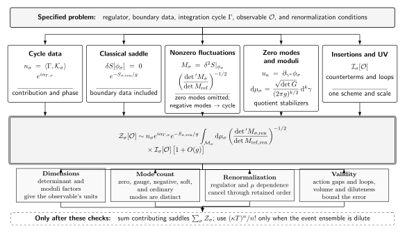
Anatomy of a regulated saddle contribution. The diagram is schematic: the determinant omits zero modes, the moduli measure replaces them, and any phase from negative directions is fixed by the integration cycle rather than by an absolute-value prescription.

The quartic double-well instanton

Take the dimensionless Euclidean action

$$S_E[x]=\frac1g\int_{-\infty}^{\infty}\mathrm d\tau\, \left[\frac12\dot x^2+\frac12(x^2-1)^2\right], \qquad g>0,$$

with $x(-\infty)=-1$ and $x(+\infty)=+1$. Completing the square gives

$$\frac12\dot x^2+\frac12(1-x^2)^2 =\frac12\bigl[\dot x-(1-x^2)\bigr]^2 +\dot x(1-x^2).$$

Therefore

$$S_E[x]\geq \frac1g\int_{-1}^{1}(1-x^2)\,\mathrm dx =\frac{4}{3g}.$$

The bound is saturated by

$$\dot x=1-x^2, \qquad x_I(\tau)=\tanh(\tau-\tau_0), \qquad S_E[x_I]=\frac{4}{3g}.$$

The one-instanton sector is consequently proportional to $e^{-4/(3g)}$. This number is the first useful control diagnostic: the dilute, leading-instanton approximation requires $4/(3g)\gg1$, not merely $g<1$. The center $\tau_0$ is an exact zero mode and cannot be included in an ordinary determinant. Multi-instanton configurations also contain separation directions that become only approximately flat; the dilute expansion additionally requires separations large compared with the core width. Coleman 1985, ch. 7, §2, pp. 270–278 and Mariño 2015, §§1.8–1.9, pp. 38–53 derive the instanton and its multi-event expansion with explicit boundary conditions.

The saddle expansion fails uniformly near a coalescence of critical points, a fluctuation eigenvalue approaching zero, or a Stokes ray. It may also fail because infrared volume factors overcome exponential suppression, because the running coupling at the saddle scale is not small, or because a nominally dilute ensemble has order-one overlap. Each is a different failure mechanism and calls for a different reorganization.

Comparison of canonical saddle calculations

The table gives a common set of checks for representative saddle problems. “Contour coefficient” records how the original integration problem selects the local Gaussian direction; it is not an instruction to replace a determinant by its absolute value. Every row ends with an observable-level control test.

Control data for canonical semiclassical saddles

Saddle	First observable	Classical action	Small parameter	Zero modes and measure	Negative modes	Determinant prescription	Contour coefficient or prescription	Renormalization	Interaction or density control	Quantitative breakdown or error test
Double-well instanton in quantum mechanics	Even–odd level splitting	4/(3g) in the normalization above	g	One translation mode with J dτ₀ per isolated event	None for the interpolating instanton	Vacuum-normalized pseudodeterminant	Fixed-endpoint real paths; unit coefficient in the one-flip sector	Only the declared quantum-mechanical normalization	κξ ≪ 1 and small connected-cluster corrections	The spectral ratio to the one-loop splitting must approach one; overlap or a soft nonzero mode invalidates the estimate
Static φ⁴ kink	Renormalized kink tension or mass	Tension times Euclidean worldvolume	Loop-counting coupling	One normalizable transverse translation mode with a center measure	None for the stable kink	Vacuum ratio per unit worldvolume	Real fields in the fixed topological sector	Vacuum counterterms in the same scheme	Kink separations large compared with the core size if a gas is formed	Box, scale, and residual renormalization dependence must be smaller than the quoted tension error
False-vacuum bounce	Decay rate per spatial volume	Bounce action minus false-vacuum action	Weak coupling or thin-wall hierarchy	d translations with the invariant center measure in d Euclidean dimensions	One radial mode for the leading bounce	Primed ratio with the negative eigenvalue treated by contour continuation	False-vacuum prescription fixes the oriented negative-mode phase and one-bounce coefficient	False-vacuum counterterms	Bounce separation large compared with radius and wall thickness	Large bounce action, exactly one negative mode, and stable determinant and volume limits; extra negative modes or gravity require a new analysis
Four-dimensional Yang–Mills instanton	Fixed-charge or θ-weighted correlator	8π²/g²(μ) plus the topological phase	Running g²(1/ρ)	d⁴x₀ dρ and gauge orientation after quotienting the stabilizer	None in the self-dual sector	Gauge-fixed nonzero-mode determinant including ghosts	Fixed-charge coefficient or eiθQ in the θ-weighted sum	Running coupling and operator renormalization	Separation much larger than size; the size distribution must be integrable in the claimed regime	ρΛ ≪ 1 and infrared convergence are required; large-size divergence or strong running coupling ends semiclassical control
Complex saddle of a regulated quartic integral	The analytically continued integral	Complex critical value	g → 0 after the quartic normalization is fixed	None away from critical-point degeneracies	Replaced by complex Morse data	Branch fixed continuously on its thimble	For positive real g, n₀=1 and n±=0 on the real cycle	No ultraviolet subtraction in zero dimensions	No event density; the relevant separation is the complex action gap	Compare the truncated saddle sum with the exact Bessel form; coalescence or an untracked Stokes jump invalidates separate Gaussian sectors

A practical control test

For a proposed saddle approximation, record the following dimensionless quantities before calculating a prefactor:

$$\frac{\operatorname{Re}(S_\tau-S_\sigma)}{g}, \qquad g\,\frac{\mathcal V_4}{\lambda_{\rm gap}^2}, \qquad \frac{\lambda_{\rm soft}}{\lambda_{\rm gap}}, \qquad \rho\,\xi .$$

They respectively probe omitted-saddle suppression, a representative interaction correction, separation of a soft eigenvalue from the ordinary spectrum, and overlap in an event ensemble of density $\rho$ and core size $\xi$. No single inequality replaces the others. A controlled claim states which of these ratios is small, over which parameter range, and what happens at its boundary.

Common pitfalls

Selecting saddles by real action alone. Critical points contribute through the integration cycle and boundary data. A lower real action does not compensate for a zero intersection number.

Calling every power series semiclassical. Loop counting follows only after a dimensionless rescaling exposes the parameter multiplying the entire action. A weak-looking coefficient in one interaction term may be offset by large fields, long distances, or a running coupling.

Hiding soft modes in the determinant. A determinant that becomes anomalously small is a warning that the Gaussian approximation is nonuniform. Promote the soft coordinate, build the appropriate uniform approximation, or restrict the stated regime.

Exercises

1. For the double well above, verify directly that differentiating the instanton gives a zero mode of the fluctuation operator.

Solution

The fluctuation operator is

$$M_I=-\frac{d^2}{d\tau^2}+V''(x_I) =-\frac{d^2}{d\tau^2}+4-6\,\operatorname{sech}^2(\tau-\tau_0).$$

Differentiate the classical equation $-\ddot x_I+V'(x_I)=0$ with respect to $\tau$. The result is $M_I\dot x_I=0$. Since $\dot x_I=\operatorname{sech}^2(\tau-\tau_0)$ is square-integrable, it is a genuine collective-coordinate zero mode.

2. Show that an $L$-loop connected vacuum graph carries $g^{L-1}$ after the rescaling $\phi=\phi_\sigma+\sqrt g\,\eta$.

Solution

A $k$-leg vertex carries $g^{k/2-1}$. With $V_k$ such vertices, the power is $\sum_k(k/2-1)V_k$. Every leg is paired in a vacuum graph, so $\sum_k kV_k=2I$. The power is therefore $I-V$, where $V=\sum_kV_k$. Connectedness gives $L=I-V+1$, hence the power $g^{L-1}$.

3. Explain why $S_I/g\gg1$ is insufficient for a dilute instanton gas.

Solution

It suppresses the fugacity of a single event but does not bound the interaction between events at the separations actually sampled. If $\kappa$ is the event fugacity and $\xi$ its core size, the mean separation is of order $\kappa^{-1}$; diluteness also requires $\kappa\xi\ll1$. Approximate separation modes and attractive instanton–anti-instanton interactions can require a correlated-event treatment even when the one-event action is large.

References

• Coleman, Sidney. Aspects of Symmetry: Selected Erice Lectures. Cambridge University Press, 1985, ch. 7, pp. 265–350. DOI.
• Mariño, Marcos. Instantons and Large N: An Introduction to Non-Perturbative Methods in Quantum Field Theory. Cambridge University Press, 2015, ch. 1, pp. 3–61. DOI.